
Log-normal distribution
The log-normal distribution is a right-skewed probability distribution of a positive variable whose natural logarithm follows a normal distribution.
Last updated: 07 Oct, 2026 · SciPy 1.18
The Normal (Gaussian) distribution is symmetric and allows negative values. Many quantities are neither: an income or the length of a comment cannot go below zero, and a few values run far to the right. The log-normal distribution describes many of them, and one log turns it back into a normal curve.
Recognising a log-normal shape
A log-normal curve has a hump on the left and a long tail on the right. The board's examples are the wealth of people and the length of comments: most people write short comments, a few write long ones, and those few stretch the tail.
In a right-skewed distribution the mode, the median and the mean come in that order, from left to right, because the long tail pulls the mean up; see Skewness and kurtosis.
Defining log-normal through the logarithm
If Y follows a normal distribution and X = eʸ, then X is log-normal. Read the other way, X is log-normal when Y = ln(X) is normal. This is the definition on the board and in the notes.
μ and σ are the mean and standard deviation of ln(X), not of X. Because X = eʸ, X is always positive. Its own centre and spread follow from μ and σ:
For μ = 0 and σ = 1 these are e^0.5 ≈ 1.6487, e⁰ = 1 and e⁻¹ ≈ 0.3679: mode below median below mean.
Turning log-normal data into normal data
The code draws 100,000 log-normal values with NumPy, takes their natural log, and compares the skewness before and after. NumPy's mean and sigma arguments are μ and σ of the log; scipy's lognorm takes σ as s and e^μ as scale.
import numpy as np
from scipy import stats

rng = np.random.default_rng(42)
x = rng.lognormal(mean=0, sigma=1, size=100_000)   # mean and sigma belong to ln(x)
y = np.log(x)                                     # natural log

print("x: smallest", round(x.min(), 4), " mean", round(x.mean(), 4), " median", round(np.median(x), 4), " skew", round(stats.skew(x), 2))
print("ln(x): mean", round(y.mean(), 4), " sd", round(y.std(), 4), " skew", round(stats.skew(y), 3))

X = stats.lognorm(s=1, scale=np.exp(0))          # s = sigma, scale = e^mu
print("formulas: mean", round(X.mean(), 4), " median", X.median(), " mode", round(np.exp(0 - 1 ** 2), 4))
print("back with exp:", np.allclose(np.exp(y), x))x: smallest 0.0124 mean 1.6517 median 0.991 skew 9.02 ln(x): mean -0.0042 sd 1.0037 skew 0.007 formulas: mean 1.6487 median 1.0 mode 0.3679 back with exp: True
Plotting log-normal data before and after the log
import numpy as np
import matplotlib.pyplot as plt
from scipy import stats

rng = np.random.default_rng(42)
x = rng.lognormal(mean=0, sigma=1, size=100_000)

fig, ax = plt.subplots(1, 2, figsize=(10, 3.6))
grid = np.linspace(0.01, 10, 500)
ax[0].hist(x, bins=100, range=(0, 10), density=True, alpha=0.6)
ax[0].plot(grid, stats.lognorm(s=1).pdf(grid), color="red")
ax[0].set_title("x is log-normal: right-skewed, x > 0")
ax[0].set_xlabel("x")
t = np.linspace(-4, 4, 400)
ax[1].hist(np.log(x), bins=60, density=True, alpha=0.6)
ax[1].plot(t, stats.norm.pdf(t), color="red")
ax[1].set_title("ln(x) is normal: N(0, 1)")
ax[1].set_xlabel("ln(x)")
fig.tight_layout()
plt.show()
print("values beyond the left plot (x > 10):", round(np.mean(x > 10), 4))values beyond the left plot (x > 10): 0.0112
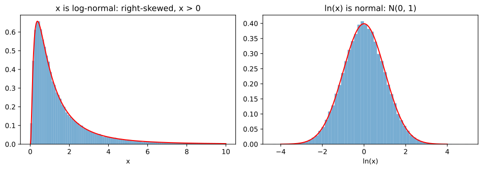
What the log shows
- Every x is positive; the smallest of 100,000 values is 0.0124.
- x is strongly right-skewed, with a skewness of 9.02 and a mean of 1.6517 well above the median of 0.991.
- ln(x) is normal: mean −0.0042, SD 1.0037 and a skewness of 0.007, close to the N(0, 1) it was built from.
- The formulas match: scipy's mean 1.6487, median 1.0 and mode 0.3679 for μ = 0, σ = 1.
- exp undoes ln: exponentiating the logs gives back the original values.
Normal vs log-normal
| Normal | Log-normal | |
|---|---|---|
| Values | Any real number | Positive only |
| Shape | Symmetric bell | Hump on the left, long right tail |
| Mean, median, mode | All equal | Mode < median < mean |
| Link | ln(X) of a log-normal X | e^Y of a normal Y |
| Typical data | Heights, measurement errors | Incomes, comment lengths, reaction times |
Where you use the log-normal distribution
- Skewed positive data: incomes for most of the population, house prices, file sizes, time spent on a page.
- Feature transformation: taking the log of a log-normal feature gives a normal one before Standardization and normalization or linear models.
- Reporting a centre: for log-normal data the median, e^μ, is a more typical value than the mean.
np.log1p(x), the log of 1 + x, avoids the error but no longer turns log-normal data into exactly normal data. The very top of a wealth distribution is also heavier-tailed than log-normal; the Pareto distribution in the next lesson fits it better.Related
- Previous: Uniform distribution
- Next: Power law and Pareto distribution
- Draw with
sigma=0.25instead of 1. Does the skewness of x fall, and do the mean and median move closer? - Use
mean=3. Is the median of x now close to e³ ≈ 20.09? - Take the log of uniform data,
np.log(rng.uniform(1, 10, 100_000)). Is the result normal? Check its skewness.
Little by little, you're building something great.