Curious builder0 XP earned · 300 to level 2

0 daysFinish a lesson to begin

Badge collection0 of 6 unlocked

57 small wins to finish your pathNext lesson →

Z-test for a proportion

A one-proportion z-test is a hypothesis test that checks whether a population proportion equals a stated value p₀, by measuring the gap between the sample proportion p̂ and p₀ in units of the standard error √(p₀(1 − p₀)/n).

Last updated: 07 Oct, 2026 · SciPy 1.18

Many questions are about a share, not a mean: the share of residents who own a phone, of users who click, of parts that are faulty. Each person answers yes or no, and the test asks whether the share of yes answers differs from a claimed value.

Setting up the cell phone problem

A problem from the notes that go with the video: a tech company believes that 70% of the residents of town XYZ own a cell phone. A marketing manager believes the share is different. A survey of 200 residents finds that 130 own one. At a 95% confidence level, is there enough evidence to reject the company's claim?

Hypotheses: H₀: p = 0.70, H₁: p ≠ 0.70 (two-tailed, since "different" allows either way).
Significance level: α = 0.05, critical values ±1.96.
Sample proportion: p̂ = x/n = 130/200 = 0.65.

Computing the z statistic for a proportion

Each answer is a Bernoulli trial, so the count of yes answers follows the Binomial distribution. For a large n the sample proportion p̂ is close to normal with mean p and standard error √(p(1 − p)/n). Under H₀, p = p₀, so the standard error uses p₀ (q₀ = 1 − p₀ is the share of no answers).

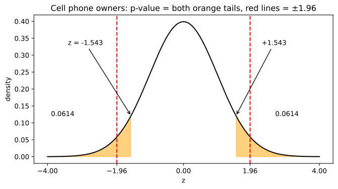
z = \frac{p ^ - p _{0}}{\frac{p _{0} ( 1 - p _{0} )}{n}} The one-proportion z statistic

z = \frac{0.65 - 0.70}{\frac{0.70 \times 0.30}{200}} = - 1.543 The cell phone survey

−1.543 lies between −1.96 and 1.96, so we fail to reject H₀. Each tail beyond |z| holds 1 − Φ(1.543) = 0.0614 of the area, so the two-tailed p-value is 2 × 0.0614 = 0.1228 > 0.05. If 70% of the town owned a phone, a survey of 200 would land at least this far from 70% about 12% of the time. The survey does not show that the share differs from 70%.

The normal approximation needs enough of both answers: n·p₀ ≥ 10 and n·(1 − p₀) ≥ 10. Here they are 140 and 60.

Running the proportion test in Python

The z statistic by hand

python

import numpy as np
from scipy.stats import norm

p0, n, x = 0.70, 200, 130            # claimed share, sample size, "yes" answers
p_hat = x / n                        # sample proportion
se = np.sqrt(p0 * (1 - p0) / n)      # standard error under H0
z = (p_hat - p0) / se

ExampleFrom the video's notes, run on SciPy 1.18.1

p_value = 2 * norm.sf(abs(z))        # two-tailed
print(f"p-hat = {p_hat}, SE = {se:.4f}, z = {z:.4f}")
print(f"critical ±{norm.ppf(0.975):.2f}, p = {p_value:.4f}")
print("reject H0" if p_value <= 0.05 else "fail to reject H0")

Output

p-hat = 0.65, SE = 0.0324, z = -1.5430
critical ±1.96, p = 0.1228
fail to reject H0

ExampleRun on matplotlib 3.11.2

import numpy as np
import matplotlib.pyplot as plt
from scipy.stats import norm

z = -1.543
x = np.linspace(-4, 4, 400)
plt.figure(figsize=(8, 4))
plt.plot(x, norm.pdf(x), color="black")
for tail in (x <= -abs(z), x >= abs(z)):                 # the p-value area
    plt.fill_between(x[tail], norm.pdf(x[tail]), color="orange", alpha=0.5)
for c in (-1.96, 1.96):
    plt.axvline(c, color="red", linestyle="--")
plt.text(-3.9, 0.12, f"{norm.sf(abs(z)):.4f}")
plt.text(2.7, 0.12, f"{norm.sf(abs(z)):.4f}")
plt.xticks([-4, -1.96, 0, 1.96, 4])
plt.annotate("z = -1.543", xy=(-1.543, 0.121), xytext=(-3.4, 0.33), arrowprops=dict(arrowstyle="->"))
plt.annotate("+1.543", xy=(1.543, 0.121), xytext=(2.3, 0.33), arrowprops=dict(arrowstyle="->"))
plt.title("Cell phone owners: p-value = both orange tails, red lines = ±1.96")
plt.xlabel("z")
plt.ylabel("density")
plt.show()
print("p-value =", round(2 * norm.sf(abs(z)), 4))

Output

p-value = 0.1228

A standard normal curve with the two orange tails beyond z = -1.543 and +1.543 shaded, 0.0614 each, inside the dashed red critical lines at -1.96 and +1.96, so the p-value 0.1228 is larger than 0.05.

The statsmodels and exact versions

statsmodels' proportions_ztest computes the standard error from p̂ unless you pass prop_var. The textbook test uses p₀, so pass prop_var=p0 to match it. SciPy's binomtest skips the normal curve and uses the binomial distribution directly.

ExampleRun on statsmodels 0.15.0 and SciPy 1.18.1

from statsmodels.stats.proportion import proportions_ztest
from scipy.stats import binomtest

z1, p1 = proportions_ztest(count=130, nobs=200, value=0.70)               # default: SE uses p-hat
z2, p2 = proportions_ztest(count=130, nobs=200, value=0.70, prop_var=0.70)  # SE uses p0
print(f"proportions_ztest default:      z = {z1:.4f}, p = {p1:.4f}")
print(f"proportions_ztest prop_var=0.7: z = {z2:.4f}, p = {p2:.4f}")
print(f"exact binomial test:            p = {binomtest(130, 200, 0.70).pvalue:.4f}")

Output

proportions_ztest default:      z = -1.4825, p = 0.1382
proportions_ztest prop_var=0.7: z = -1.5430, p = 0.1228
exact binomial test:            p = 0.1234

What the three versions agree on

With the SE from p₀, z = −1.5430 and p = 0.1228, the textbook values above.
The default SE from p̂ gives z = −1.4825 and p = 0.1382. A different standard error, so a slightly different number.
The exact binomial test gives p = 0.1234. All three fail to reject H₀ at α = 0.05; with n = 200 the normal approximation is close to the exact answer.

Testing one direction: the car ownership problem

The notes' second problem: a car company believes that 60% or less of the residents of city ABC own a vehicle. A sales manager disagrees. A survey of 250 residents finds 170 who own one. At a 10% significance level, is there enough evidence against the company's claim?

Hypotheses: H₀: p ≤ 0.60 (the claim, with the equality), H₁: p > 0.60. Only a high share counts against H₀, so the test is right-tailed.
Statistic: p̂ = 170/250 = 0.68 and z = (0.68 − 0.60)/√(0.6 × 0.4/250) = 2.582.
Decision: the one-tailed critical value at α = 0.10 is 1.282, and p = P(Z ≥ 2.582) = 0.0049. Reject H₀: the survey is evidence that more than 60% of residents own a vehicle.

ExampleFrom the video's notes, run on SciPy 1.18.1

import numpy as np
from scipy.stats import norm

p0, n, x, alpha = 0.60, 250, 170, 0.10
p_hat = x / n
z = (p_hat - p0) / np.sqrt(p0 * (1 - p0) / n)
p_value = norm.sf(z)                  # upper tail only: H1 is p > 0.60
print(f"p-hat = {p_hat}, z = {z:.3f}, critical = {norm.ppf(1 - alpha):.3f}, p = {p_value:.4f}")
print("reject H0" if p_value <= alpha else "fail to reject H0")

Output

p-hat = 0.68, z = 2.582, critical = 1.282, p = 0.0049
reject H0