
Confidence intervals
A confidence interval is a range computed from a sample as point estimate ± margin of error, by a procedure that captures the true population parameter in a stated share of repeated samples (the confidence level).
Last updated: 07 Oct, 2026 · SciPy 1.18
The Point estimates and standard error lesson ended with x̄ and its standard error. A confidence interval turns the two into a range of plausible values for μ, with a stated level of confidence.
Setting up the CAT score question
The video's question: on the quant test of the CAT exam, the population standard deviation is known to be 100. A sample of 25 test takers has a mean score of 520. Construct a 95% confidence interval for the mean.
- Given: σ = 100, n = 25, x̄ = 520.
- Confidence level 95%, so α = 1 − 0.95 = 0.05. The confidence level is always 1 − α.
- Two tails: the interval leaves α/2 = 0.025 outside each end.
Because σ is known, the margin of error uses the z critical value zα/2 and the standard error σ/√n:
Building a 95% z-interval
The interval splits into an upper and a lower limit. For z0.025, the z-table is read at a left area of 1 − 0.025 = 0.975: row 1.9, column 0.06, so z0.025 = 1.96. The standard error is 100/√25 = 20.
So the 95% confidence interval for the mean quant score is 480.8 to 559.2, centred on the point estimate 520. The z-interval needs σ to be known, and either normally distributed scores or a sample large enough for the central limit theorem; with normal scores, n = 25 is fine. The Z-table and normal probabilities lesson covers reading the table.
import numpy as np
import matplotlib.pyplot as plt
from scipy.stats import norm

x = np.linspace(440, 600, 400)
y = norm.pdf(x, loc=520, scale=20)        # x̄ ± its standard error of 20
lo, hi = norm.interval(0.95, loc=520, scale=20)
plt.figure(figsize=(8, 4))
plt.plot(x, y, color="black")
plt.fill_between(x, y, where=(x >= lo) & (x <= hi), alpha=0.3, label="central 95%")
for v in (lo, 520, hi):
    plt.axvline(v, color="red" if v != 520 else "grey", linestyle="--")
plt.title("95% z-interval for the CAT mean: 520 ± 1.96 × 20")
plt.xlabel("score")
plt.ylabel("density")
plt.legend()
plt.show()
print("limits:", round(lo, 1), "and", round(hi, 1))limits: 480.8 and 559.2
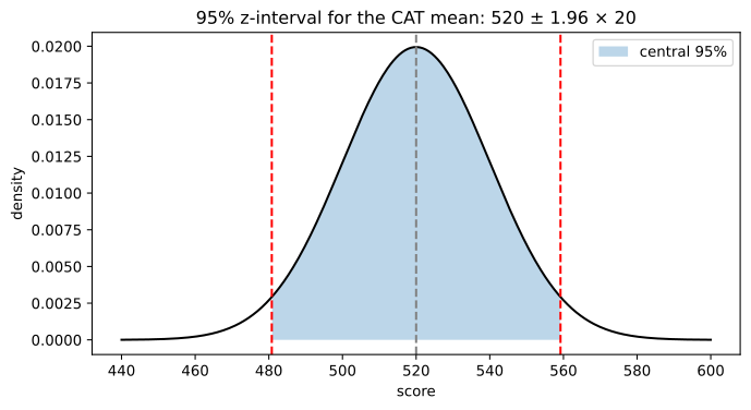
The curve is the sampling distribution of x̄ with SE 20, drawn around the estimate 520. It describes sample means, not single CAT scores, which spread five times wider.
Building a 95% t-interval when σ is unknown
The video's second question changes one fact: the same 25 test takers have mean 520 and a sample standard deviation s = 80, and the population SD is not given. With σ unknown and estimated by s, the critical value comes from the t distribution with n − 1 degrees of freedom:
Degrees of freedom: n − 1 = 25 − 1 = 24, the same n − 1 as in the sample variance. The t-table at df 24 and a one-tail area of 0.025 (two tails 0.05) gives 2.064. The standard error is 80/√25 = 16.
To two decimals the interval is 486.98 to 553.02. The t critical value 2.064 is larger than 1.96 because s is itself an estimate; the extra width pays for that uncertainty, and t approaches z as n grows. The One-sample t-test and the t distribution lesson covers the t distribution.
Computing both intervals in Python
norm.ppf(0.975) and t.ppf(0.975, df=24) replace the two table look-ups. SciPy can also return the limits in one call: norm.interval(0.95, loc=520, scale=20) and t.interval(0.95, df=24, loc=520, scale=16).
import numpy as np
from scipy.stats import norm, t

xbar, n = 520, 25

# z-interval: the population SD sigma = 100 is known
z = norm.ppf(0.975)                  # area 0.975 to the left: the 1.96 of the z-table
se = 100 / np.sqrt(n)
print(f"z = {z:.4f}, SE = {se:.0f}, 95% z-interval: {xbar - z * se:.2f} to {xbar + z * se:.2f}")

# t-interval: only the sample SD s = 80 is known, df = n - 1 = 24
tc = t.ppf(0.975, df=n - 1)
se = 80 / np.sqrt(n)
print(f"t = {tc:.4f}, SE = {se:.0f}, 95% t-interval: {xbar - tc * se:.2f} to {xbar + tc * se:.2f}")
print(f"with the table's t = 2.064: {xbar - 2.064 * se:.3f} to {xbar + 2.064 * se:.3f}")z = 1.9600, SE = 20, 95% z-interval: 480.80 to 559.20 t = 2.0639, SE = 16, 95% t-interval: 486.98 to 553.02 with the table's t = 2.064: 486.976 to 553.024
- The z-interval is 480.80 to 559.20, as on the board, with z = 1.9600 and SE 20.
- The t-interval is 486.98 to 553.02 with the exact t = 2.0639; the table's 2.064 gives 486.976 to 553.024.
- The t-interval is narrower here only because s = 80 is smaller than σ = 100. With the same SD, the t-interval is always the wider one.
Reading a 95% confidence level correctly
A 95% confidence interval comes from a procedure that, over repeated samples, produces intervals containing the true μ 95% of the time. The 95% describes the method. Any one computed interval, such as 480.8 to 559.2, either contains μ or it does not; it is not true that μ lies inside it with probability 95%. The interval also says nothing about where 95% of individual scores fall.
A simulation makes this visible. The code below fixes the true mean at μ = 500 (σ = 100), draws 1,000 samples of 25, builds a 95% t-interval from each, and counts how many intervals contain 500.
import numpy as np
import matplotlib.pyplot as plt
from scipy import stats

rng = np.random.default_rng(42)
mu, sigma, n = 500, 100, 25          # the true mean is known here, so hits can be counted
intervals = []
for i in range(1000):
    s = rng.normal(mu, sigma, n)
    intervals.append(stats.t.interval(0.95, df=n - 1, loc=s.mean(), scale=stats.sem(s)))
hits = [lo <= mu <= hi for lo, hi in intervals]
print("intervals that contain mu = 500:", sum(hits), "of 1000")
print("misses among the first 50 drawn:", 50 - sum(hits[:50]))

plt.figure(figsize=(8, 5))
for i, (lo, hi) in enumerate(intervals[:50]):
    plt.plot([lo, hi], [i, i], color="tab:blue" if hits[i] else "red", linewidth=2)
plt.axvline(mu, color="black", linestyle="--")
plt.title("50 samples of 25, one 95% t-interval each (red misses mu = 500)")
plt.xlabel("score")
plt.ylabel("sample")
plt.show()intervals that contain mu = 500: 948 of 1000 misses among the first 50 drawn: 3
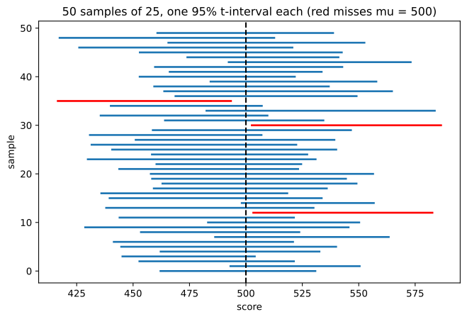
What the coverage simulation shows
- 948 of the 1,000 intervals contain μ: a coverage of 0.948, close to the promised 0.95. A longer run settles nearer to 0.95.
- Each interval is different, because each sample has its own x̄ and s. Some are wider, some narrower.
- 3 of the first 50 intervals miss (drawn in red). Nothing in a single interval says whether it is one of the misses, which is why the 95% belongs to the method and not to one interval.
Changing the width of a confidence interval
Three things set the width 2 × critical value × SE: the confidence level (a larger level needs a larger critical value), the spread σ, and the sample size n. The last line answers a planning question: how many test takers give a margin of error of ±10 points at 95%? Solving E = z σ/√n for n gives n = (z σ / E)².
import math
from scipy.stats import norm

sigma = 100
for conf in (0.90, 0.95, 0.99):
    z = norm.ppf(1 - (1 - conf) / 2)
    print(f"{conf:.0%}: z = {z:.3f}, width with n = 25: {2 * z * sigma / math.sqrt(25):.1f}, "
          f"with n = 100: {2 * z * sigma / math.sqrt(100):.1f}")

E = 10                                   # the margin of error wanted: ±10 points
n_needed = (norm.ppf(0.975) * sigma / E) ** 2
print("n for a ±10 margin at 95%:", round(n_needed, 2), "-> round up to", math.ceil(n_needed))90%: z = 1.645, width with n = 25: 65.8, with n = 100: 32.9 95%: z = 1.960, width with n = 25: 78.4, with n = 100: 39.2 99%: z = 2.576, width with n = 25: 103.0, with n = 100: 51.5 n for a ±10 margin at 95%: 384.15 -> round up to 385
- Higher confidence gives a wider interval: with n = 25 the width grows from 65.8 (90%) to 78.4 (95%) and 103.0 (99%).
- Four times the data halves the width: 78.4 becomes 39.2 at 95%.
- A ±10 margin needs n = 385: (1.96 × 100 / 10)² = 384.15, rounded up. This is how the video's interview question about the average size of sharks is answered in practice: decide the margin, use a pilot estimate of σ, and compute the sample size before collecting data.
z-interval vs t-interval
| z-interval | t-interval | |
|---|---|---|
| When | σ known (normal data or large n) | σ unknown, estimated by s |
| Formula | x̄ ± zα/2 σ/√n | x̄ ± tα/2, n−1 s/√n |
| Critical value at 95% | 1.96 | 2.064 for df 24, closer to 1.96 as n grows |
| CAT example | 480.8 to 559.2 | 486.98 to 553.02 |
| SciPy | norm.interval(0.95, loc, scale) | t.interval(0.95, df, loc, scale) |
Where you use confidence intervals
- Reporting an estimate: an average order value of ₹1,250 with a 95% CI of ₹1,180 to ₹1,320 says how precise the number is.
- A/B tests: a CI for the difference between two conversion rates shows the size of the effect, not only whether there is one.
- Planning a study: the sample size for a target margin of error, n = (z σ / E)².
Related
- Previous: Point estimates and standard error
- Next: Hypothesis testing
- Reference: scipy.stats.t
- Change the confidence level to 99% in the CAT example (
0.995in bothppfcalls). How much wider does each interval get? - In the coverage simulation, use
stats.t.interval(0.90, ...). Does the count drop to about 900? - Set
E = 5in the width example. Why does halving the margin of error need four times the sample?
Every expert started right here.