
Choosing a statistical test
Choosing a statistical test is the step of matching a question to the test whose assumptions fit it, decided by the type of data, the number of groups, whether the groups are paired and what is known about the population.
Last updated: 07 Oct, 2026 · SciPy 1.18
The video's interview advice is to know why a test is used. This lesson puts the tests from the previous lessons side by side, adds the rank-based alternatives, and covers two things a p-value does not tell you: how big the effect is, and what happens when you run many tests.
Asking four questions about the data
- What type is the variable? Numeric values call for tests on means; categories call for tests on counts and proportions (see Types of variables).
- How many groups? One group against a stated value, two groups, or three and more.
- Are the groups independent or paired? Different subjects, or the same subjects measured twice.
- What is known or assumed? A known σ, roughly normal data, a large enough sample, expected counts of at least 5.
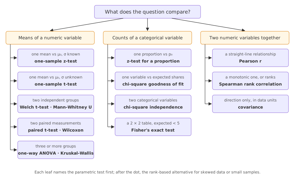
Matching each test to its example
| Question | Data | Test | SciPy / statsmodels |
|---|---|---|---|
| Did the medication change mean IQ? (σ = 15 known) | numeric, 1 group | One-sample z-test | by hand with norm |
| Same, with only the sample s = 20 | numeric, 1 group | One-sample t-test and the t distribution | ttest_1samp |
| Do class A and class B have the same mean age? | numeric, 2 independent groups | Two-sample and paired t-tests | ttest_ind(equal_var=False) |
| Did weights change between week 10 and week 20? | numeric, paired | Paired t-test | ttest_rel |
| Do 70% of residents own a phone? | yes/no, 1 group | Z-test for a proportion | proportions_ztest, binomtest |
| Has the age mix changed since 2000? | 1 categorical variable | Chi-square goodness-of-fit test | chisquare |
| Is smoking related to sex? | 2 categorical variables | Chi-square test of independence | chi2_contingency |
| Do 3 iris species share a mean petal width? | numeric, 3 groups | One-way ANOVA (F-test) | f_oneway |
Choosing parametric or non-parametric tests
A parametric test assumes a form for the population, usually normal, and tests a parameter such as the mean: z, t and ANOVA. A non-parametric test makes no such assumption. The rank-based ones replace the values by their ranks, so outliers and skew matter less; they test whether one group tends to have larger values than another. Use them for small, skewed or ordinal data, and for data with outliers.
| Parametric test | Rank-based alternative | SciPy |
|---|---|---|
| One-sample or paired t-test | Wilcoxon signed-rank test | wilcoxon |
| Two-sample t-test | Mann-Whitney U test | mannwhitneyu |
| One-way ANOVA | Kruskal-Wallis H test | kruskal |
| Pearson correlation | Spearman rank correlation | spearmanr |
On the notebook's class ages both kinds of test agree:
import numpy as np
from scipy import stats

np.random.seed(6)
school_ages = stats.poisson.rvs(loc=18, mu=35, size=1500)
classA_ages = stats.poisson.rvs(loc=18, mu=30, size=60)
np.random.seed(12)
ClassB_ages = stats.poisson.rvs(loc=18, mu=33, size=60)
print("Welch t-test p:  ", round(stats.ttest_ind(classA_ages, ClassB_ages, equal_var=False).pvalue, 6))
print("Mann-Whitney U p:", round(stats.mannwhitneyu(classA_ages, ClassB_ages).pvalue, 6))Welch t-test p: 0.000399 Mann-Whitney U p: 0.001317
The p-values differ in size but both are below 0.05, so both reject H₀. When the data are close to normal, the two kinds of test usually agree; they part ways when outliers or heavy skew are present.
Measuring the effect size
A p-value says whether a difference is likely to be more than sampling noise. It does not say how big the difference is. An effect size does: Cohen's d is the difference in means in units of the standard deviation, and Cramér's V runs from 0 (no association) to 1 for a contingency table.
import numpy as np
import pandas as pd
import seaborn as sns
from scipy import stats

d_iq = (140 - 100) / 15                                   # Cohen's d, the z-test example
x = np.array([88, 92, 94, 94, 96, 97, 97, 97, 99, 99,
              105, 109, 109, 109, 110, 112, 112, 113, 114, 115])
d_20 = (x.mean() - 100) / x.std(ddof=1)                   # Cohen's d, the 20 patients
tips = sns.load_dataset("tips")
table = pd.crosstab(tips["sex"], tips["smoker"])
chi2 = stats.chi2_contingency(table, correction=False).statistic
cramers_v = np.sqrt(chi2 / (table.values.sum() * (min(table.shape) - 1)))
print("Cohen's d, IQ 140 vs 100:", round(d_iq, 2))
print("Cohen's d, 20 patients:  ", round(d_20, 2))
print("Cramer's V, sex by smoker:", round(cramers_v, 4))Cohen's d, IQ 140 vs 100: 2.67 Cohen's d, 20 patients: 0.36 Cramer's V, sex by smoker: 0.0028
A d of 2.67 is a huge effect: the medication group sits 2.67 population standard deviations above the norm. The 20 patients' d of 0.36 is small to moderate, and Cramér's V of 0.0028 for sex by smoking is essentially no association. The opposite also happens: with a very large sample a tiny difference becomes "significant".
import numpy as np
from scipy import stats

rng = np.random.default_rng(42)
a = rng.normal(loc=100.0, scale=15, size=200_000)
b = rng.normal(loc=100.3, scale=15, size=200_000)      # a 0.3-point true difference
r = stats.ttest_ind(a, b, equal_var=False)
d = (b.mean() - a.mean()) / np.sqrt((a.var(ddof=1) + b.var(ddof=1)) / 2)
print(f"p = {r.pvalue:.2g}, Cohen's d = {d:.3f}")p = 9.2e-12, Cohen's d = 0.022
With 200,000 people per group, a 0.3-point IQ difference gives a p-value far below 0.05, but d is about 0.02, too small to matter for any decision. Report the effect size next to the p-value.
Correcting for multiple tests
Every test at α = 0.05 has a 5% chance of a Type I error when H₀ is true (see Type I and Type II errors). Run 20 independent tests on data with no real effects and the chance of at least one false alarm is 1 − 0.95²⁰ = 0.642. The Bonferroni correction divides α by the number of tests m, so each test uses α/m and the chance of any false alarm stays at most α.
import numpy as np
from scipy import stats

alpha, m = 0.05, 20
print("P(at least one false alarm in 20 tests):", round(1 - (1 - alpha) ** m, 3))
rng = np.random.default_rng(42)
p_values = [stats.ttest_ind(rng.normal(size=30), rng.normal(size=30)).pvalue for _ in range(m)]
p_values = np.array(p_values)                            # H0 is true in every test
print("tests with p <= 0.05:         ", int((p_values <= alpha).sum()))
print("tests with p <= 0.05/20:      ", int((p_values <= alpha / m).sum()))
print("smallest p:", round(p_values.min(), 4))P(at least one false alarm in 20 tests): 0.642 tests with p <= 0.05: 1 tests with p <= 0.05/20: 0 smallest p: 0.0327
In this run of 20 tests where H₀ is true every time, one test still came out below 0.05, while none passed the Bonferroni threshold 0.05/20 = 0.0025. A/B testing tools that compare many metrics or many variants need this kind of correction.
Where you use the test checklist
- Interviews: "which test would you use?" questions are answered with the four questions above, then the assumptions you would check.
- A/B tests: a t-test (or Mann-Whitney U) on time spent and a chi-square or proportion test on conversions, with an effect size and a multiple-testing correction when many metrics are compared.
- Data analysis reports: name the test, its assumptions, the statistic, the p-value and the effect size.
Related
- Previous: One-way ANOVA (F-test)
- Next: Covariance
- See also: Hypothesis testing, P-value
- Reference: SciPy hypothesis tests
- Run
stats.wilcoxonon the paired weights from Two-sample and paired t-tests and compare its p-value with the paired t-test's 0.5732. - In the large-sample example change
size=200_000tosize=200. Is the 0.3-point difference still significant? - Change
m = 20tom = 100in the multiple-testing example. How many false alarms appear at 0.05?
You understood something today that you didn't yesterday.