
Standardization and normalization
Standardization and normalization are feature scaling methods that put columns measured in different units on one common scale: standardization turns each value into its z-score, so a column gets mean 0 and standard deviation 1, and min-max normalization maps each column onto the range 0 to 1.
Last updated: 07 Oct, 2026 · SciPy 1.18
Z-score and the standard normal distribution measured one value in standard deviations. Machine learning does the same to whole columns, because columns in years, rupees and kilograms cannot be compared as raw numbers.
Seeing why columns need scaling
The video's practical application is a machine learning dataset with three features: age in years (24, 25, 26, 27), salary in rupees (40K, 80K, 60K, 70K) and weight in kilograms (70, 80, 55, 45). The units differ, and so do the sizes: a difference of 1 in salary is one rupee, a difference of 1 in age is a whole year. A model that measures distances between rows, such as K nearest neighbours (KNN), would be driven almost entirely by salary.
Standardizing each column with the z-score
Standardization applies the z-score to every value of a column, using that column's own mean and standard deviation:
Every standardized column has mean 0 and standard deviation 1, whatever its units. Age 24 becomes −1.3416: 1.34 standard deviations below the mean age of 25.5. The σ here is the population standard deviation (divide by n), the convention scikit-learn's StandardScaler uses.
Normalizing to 0 to 1 with min-max scaling
Normalization, as the video uses the word, moves the values into a range you choose, usually 0 to 1 and sometimes −1 to 1. The tool for it is the min-max scaler:
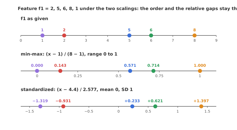
The smallest value becomes 0 and the largest becomes 1. For a range from a to b the formula is x' = a + (x − min)(b − a)/(max − min). In the notes that go with the video, the feature f1 = 2, 5, 6, 8, 1 has min 1 and max 8, so 2 becomes (2 − 1)/(8 − 1) = 1/7 = 0.143, 5 becomes 4/7 = 0.571, 6 becomes 5/7 = 0.714, 8 becomes 1 and 1 becomes 0.
The video's deep learning case is images. A CNN for image classification takes pixels from 0 to 255, and before training each pixel is divided by 255, so 0 stays 0 and 255 becomes 1. That is min-max scaling with the bounds fixed at the pixel range instead of read from the image; when an image holds both a 0 and a 255 pixel, the two give the same numbers.
The word normalization has other meanings too. scikit-learn's Normalizer rescales each row to length 1, which is a different operation, so "min-max scaling" is the clearer name for this one.
Scaling the age, salary and weight table
Standardizing with pandas
pandas .std() divides by n − 1 by default (ddof=1). ddof=0 divides by n, the same as numpy and StandardScaler.
standardized = (df - df.mean()) / df.std(ddof=0) # z-score per column, divide by nMin-max scaling with pandas
minmax = (df - df.min()) / (df.max() - df.min()) # each column onto 0 to 1import pandas as pd
df = pd.DataFrame({"age": [24, 25, 26, 27],
"salary": [40_000, 80_000, 60_000, 70_000],
"weight": [70, 80, 55, 45]})
standardized = (df - df.mean()) / df.std(ddof=0)
minmax = (df - df.min()) / (df.max() - df.min())
print(standardized.round(4))
print(minmax.round(4))
print("means after standardizing:", standardized.mean().round(4).tolist())
print("SDs after standardizing: ", standardized.std(ddof=0).round(4).tolist()) age salary weight
0 -1.3416 -1.5213 0.5571
1 -0.4472 1.1832 1.2999
2 0.4472 -0.1690 -0.5571
3 1.3416 0.5071 -1.2999
age salary weight
0 0.0000 0.00 0.7143
1 0.3333 1.00 1.0000
2 0.6667 0.50 0.2857
3 1.0000 0.75 0.0000
means after standardizing: [0.0, 0.0, 0.0]
SDs after standardizing: [1.0, 1.0, 1.0]What the scaled table shows
- Standardized age is −1.3416, −0.4472, 0.4472, 1.3416: evenly spaced ages stay evenly spaced.
- Standardized salary is −1.5213, 1.1832, −0.169, 0.5071: 80K is 1.18 SDs above the mean of 62,500, and the rupee figures are now on the same footing as age and weight.
- Every standardized column has mean 0.0 and SD 1.0.
- Min-max salary is 0.0, 1.0, 0.5, 0.75: 40K, the smallest, becomes 0 and 80K, the largest, becomes 1. Weight becomes 0.7143, 1.0, 0.2857, 0.0.
Standardization keeps the shape of the data
Standardizing changes the numbers on the axis, never the shape of the distribution. The tips bills from the video's Python session show it:
import matplotlib.pyplot as plt
import seaborn as sns
from scipy.stats import skew

bill = sns.load_dataset("tips")["total_bill"]
z = (bill - bill.mean()) / bill.std(ddof=0)

fig, axes = plt.subplots(1, 2, figsize=(10, 4))
axes[0].hist(bill, bins=20, color="steelblue", edgecolor="white")
axes[0].set_title("total_bill in dollars")
axes[1].hist(z, bins=20, color="seagreen", edgecolor="white")
axes[1].set_title("total_bill standardized")
plt.show()
print("skewness before:", round(skew(bill), 3), " after:", round(skew(z), 3))
print("range before:", bill.min(), "to", bill.max(), " after:", round(z.min(), 3), "to", round(z.max(), 3))skewness before: 1.126 after: 1.126 range before: 3.07 to 50.81 after: -1.882 to 3.492
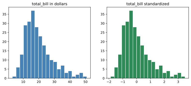
The two histograms are the same picture with a new axis, and the skewness is 1.126 before and after. Standardized data has mean 0 and SD 1, but it is not standard normal unless the original column was normal.
Min-max scaling and outliers
The outlier dataset from Outlier detection with IQR and z-score has 31 values between 10 and 19 and three far above them:
import numpy as np

dataset = np.array([11, 10, 12, 14, 12, 15, 14, 13, 15, 102, 12, 14, 17, 19, 107,
                    10, 13, 12, 14, 12, 108, 12, 11, 14, 13, 15, 10, 15, 12, 10, 14, 13, 15, 10])
scaled = (dataset - dataset.min()) / (dataset.max() - dataset.min())
print("min-max of 102, 107, 108:", scaled[dataset > 100].round(3))
print("largest of the other 31: ", scaled[dataset < 100].max().round(3))
print("share of values below 0.1:", np.mean(scaled < 0.1).round(3))min-max of 102, 107, 108: [0.939 0.99 1. ] largest of the other 31: 0.092 share of values below 0.1: 0.912
The three outliers take the top of the range and squeeze the other 31 values into 0 to 0.092, so 91.2% of the data ends up below 0.1. Outliers also inflate the standard deviation that standardization divides by, so handle them before scaling.
Fitting the scaler on the training data only
In a machine learning pipeline, scikit-learn's StandardScaler and MinMaxScaler apply these two formulas. The mean, SD, min and max must come from the training rows only, and the test rows are then transformed with those same numbers. Fitting on all the rows lets the test set leak into training and makes the test score look better than it will be on new data. Train and test split covers the split itself.
from sklearn.model_selection import train_test_split
from sklearn.preprocessing import MinMaxScaler, StandardScaler

X_train, X_test = train_test_split(df, test_size=0.25, random_state=42)
scaler = StandardScaler()                          # or MinMaxScaler()
X_train_scaled = scaler.fit_transform(X_train)     # learns mean and SD from train
X_test_scaled = scaler.transform(X_test)           # reuses them on test
StandardScaler divides by the population standard deviation, the same as ddof=0 above, so on the training rows it gives the numbers the pandas formula gives.
Standardization vs normalization
| Standardization | Min-max normalization | |
|---|---|---|
| Formula | (x − μ)/σ | (x − min)/(max − min) |
| Result | Mean 0, SD 1, no fixed range | Range 0 to 1, or a range you choose |
| Shape of the data | Unchanged | Unchanged |
| Outliers | Inflate σ and pull the other values together | Squeeze the other values into a small part of the range |
| scikit-learn | StandardScaler | MinMaxScaler |
| Typical use | Linear and logistic regression, SVM, PCA, KNN, k-means | Image pixels for CNNs, inputs that must stay bounded |
Where you use standardization and normalization
- Distance-based models. KNN and k-means compare rows by distance, so every feature must be on one scale; see K nearest neighbours (KNN).
- Gradient descent. Features on similar scales let Gradient descent move evenly in every direction instead of zigzagging.
- Images. Pixels are divided by 255 before a CNN is trained, as in the video.
Related
- Previous: Z-score and the standard normal distribution
- Next: Z-table and normal probabilities
- See also: Outlier detection with IQR and z-score
- See also: Train and test split
- Reference: scikit-learn preprocessing
- Replace
df.std(ddof=0)with the pandas defaultdf.std()in the table example: age 24 becomes −1.1619 instead of −1.3416. - Scale salary to the range −1 to 1 with
-1 + 2 * minmax["salary"]: 40K becomes −1, 60K becomes 0 and 80K becomes 1. - Drop 102, 107 and 108 from
dataset(dataset[dataset < 100]) and min-max scale again: the 31 values now spread over the whole range, and the four 13s sit at 0.333.
Slow is fine. Stopping is the only problem.