
Empirical rule (68-95-99.7)
The empirical rule (the 68-95-99.7 rule) is a property of the normal distribution: about 68% of the values lie within one standard deviation of the mean, about 95% within two, and about 99.7% within three.
Last updated: 07 Oct, 2026 · SciPy 1.18
Normal (Gaussian) distribution marked the bell curve in steps of one standard deviation. The empirical rule says how much of the data sits between those steps, without any calculation.
Reading the three bands
The video's example is a dataset of 100 data points that follows a normal distribution. Within one standard deviation of the mean, from μ − σ to μ + σ, lies about 68% of the data, so about 68 of the 100 points. That central region holds most of the data, which is what gives the curve its bell shape.
Within two standard deviations, μ − 2σ to μ + 2σ, lies about 95% of the data, and within three, μ − 3σ to μ + 3σ, about 99.7%. The rule is also called the three-sigma rule. The exact areas are 68.27%, 95.45% and 99.73%:
The 68 out of 100 is what you expect on average. A real sample of 100 points lands near 68, not exactly on it, as the simulation further down shows.
The video's real-world example is height. A doctor, the domain expert here, measures people from many places, draws the bell curve and reads off how much of the data falls within one, two and three standard deviations. Heights within one group, such as adult women of one country, are close to normal, so the rule works for them.
Drawing the bands for mean 4 and SD 1
The share within k standard deviations
The area between −k and +k on the standard normal curve is the same for every normal distribution, so one line gives each band.
from scipy.stats import norm

k = 2
norm.cdf(k) - norm.cdf(-k) # share within k standard deviations of the meanimport numpy as np
import matplotlib.pyplot as plt
from scipy.stats import norm
mu, sigma = 4, 1 # the video's mean and SD
x = np.linspace(mu - 4 * sigma, mu + 4 * sigma, 400)
plt.figure(figsize=(8, 4))
plt.plot(x, norm.pdf(x, mu, sigma), color="black")
for k, color in [(1, "red"), (2, "blue"), (3, "green")]:
share = norm.cdf(k) - norm.cdf(-k)
ring = (np.abs(x - mu) <= k * sigma) & (np.abs(x - mu) >= (k - 1) * sigma)
plt.fill_between(x, norm.pdf(x, mu, sigma), where=ring, color=color, alpha=0.35,
label=f"{mu - k * sigma} to {mu + k * sigma}: {share:.2%}")
print(f"within {k} SD ({mu - k * sigma} to {mu + k * sigma}): {share:.4f}")
plt.title("Empirical rule for mean 4 and SD 1")
plt.xlabel("x")
plt.legend()
plt.show()within 1 SD (3 to 5): 0.6827 within 2 SD (2 to 6): 0.9545 within 3 SD (1 to 7): 0.9973
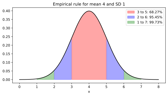
Red, blue and green mark one, two and three standard deviations, the colours of the board in the video. With mean 4 and SD 1, about 68% of values lie between 3 and 5, 95% between 2 and 6, and 99.7% between 1 and 7.
Checking the rule on simulated samples
Draw values from N(4, 1) with numpy and count how many fall within one, two and three of the sample's own standard deviations of its own mean. x.std() divides by n (ddof = 0); with 100 or more values the choice hardly matters here.
import numpy as np

rng = np.random.default_rng(42)
for n in [100, 10_000]:
    x = rng.normal(loc=4, scale=1, size=n)          # n draws from N(4, 1)
    m, s = x.mean(), x.std()                        # the sample's own mean and SD
    shares = [np.mean(np.abs(x - m) <= k * s) * 100 for k in (1, 2, 3)]
    print(f"n = {n:6}: mean {m:.3f}, SD {s:.3f}, within 1/2/3 SD: "
+ " / ".join(f"{v:.1f}%" for v in shares))n = 100: mean 3.950, SD 0.773, within 1/2/3 SD: 65.0% / 96.0% / 100.0% n = 10000: mean 3.989, SD 1.009, within 1/2/3 SD: 68.1% / 95.5% / 99.7%
What the simulated shares show
- The 100-point sample gives 65.0%, 96.0% and 100.0%: near 68, 95 and 99.7, not on them. Its mean 3.950 and SD 0.773 also miss the true 4 and 1, because 100 values carry sampling noise.
- The 10,000-point sample gives 68.1%, 95.5% and 99.7%, with mean 3.989 and SD 1.009: a large sample from a normal distribution follows the rule closely.
- So "68 of 100 points" is an expected count. Any one dataset of 100 normal values scatters around it.
Chebyshev's inequality for any distribution
The empirical rule needs a normal distribution. For any distribution with a finite standard deviation, Chebyshev's inequality gives a floor that always holds:
With k = 2, at least 75% of the values lie within two standard deviations; with k = 3, at least 88.9%. The floor is low, but it never fails. For k = 1 it says nothing, since 1 − 1/1 = 0.
The restaurant bills from the video's Python session (the seaborn tips data) have a long right tail, so they make a fair test:
import numpy as np
import seaborn as sns
from scipy.stats import norm

bill = sns.load_dataset("tips")["total_bill"]      # 244 restaurant bills
m, s = bill.mean(), bill.std(ddof=0)
for k in (1, 2, 3):
    share = np.mean(np.abs(bill - m) <= k * s)
    print(f"within {k} SD: tips {share:.1%}   normal {norm.cdf(k) - norm.cdf(-k):.1%}   "
f"Chebyshev at least {1 - 1 / k**2:.1%}")within 1 SD: tips 72.1% normal 68.3% Chebyshev at least 0.0% within 2 SD: tips 94.3% normal 95.4% Chebyshev at least 75.0% within 3 SD: tips 98.4% normal 99.7% Chebyshev at least 88.9%
The bills are skewed, so the normal shares fit them only roughly: 72.1% within one SD instead of 68.3%, 98.4% within three instead of 99.7%. Chebyshev's floors of 75.0% and 88.9% hold, as they always do. The SD here divides by n (ddof=0).
Following the rule does not prove normality
In the video a viewer asks whether data that follows the empirical rule must be normally distributed. The direction that holds is the other one: normal data follows the rule. A distribution that is not normal can still come close to 68, 95 and 99.7, so matching the rule is a quick sanity check, not a proof. To check normality, use a Q-Q plot or a test, as in Normality tests (Q-Q plot and Shapiro-Wilk).
Empirical rule vs Chebyshev's inequality
| Empirical rule | Chebyshev's inequality | |
|---|---|---|
| Works for | Normal distributions only | Any distribution with a finite standard deviation |
| Within 1 SD | About 68% (68.27%) | No guarantee |
| Within 2 SD | About 95% (95.45%) | At least 75% |
| Within 3 SD | About 99.7% (99.73%) | At least 88.9% |
| Kind of statement | About this share | At least this share |
Where you use the empirical rule
- Quick ranges. With mean 4 and SD 1, about 95% of values lie between 2 and 6, with no table.
- Flagging outliers. Only 0.27% of a normal population lies beyond three standard deviations, the reason for the |z| > 3 rule in Outlier detection with IQR and z-score.
- Quality control. Control charts draw limits at μ ± 3σ; a point outside them is rare enough under normal running to call for a look.
- Intervals. The exact multiplier for 95% is 1.96, not 2; Confidence intervals uses it.
Related
- Previous: Normal (Gaussian) distribution
- Next: Z-score and the standard normal distribution
- See also: Outlier detection with IQR and z-score
- Reference: scipy.stats.norm
- In the simulation, change the seed from 42 to 7: the 100-point shares move to different values near 68, 95 and 99.7, while the 10,000-point shares stay within a few tenths of a percent of them.
- Change
(1, 2, 3)to(1.5, 2.5)in the tips loop: Chebyshev's floors become 55.6% and 84.0%. - Replace
rng.normal(loc=4, scale=1, size=n)withrng.exponential(scale=1, size=n): the within-1-SD share of the large sample rises to about 86%, far from 68%.
Little by little, you're building something great.