
Uniform distribution
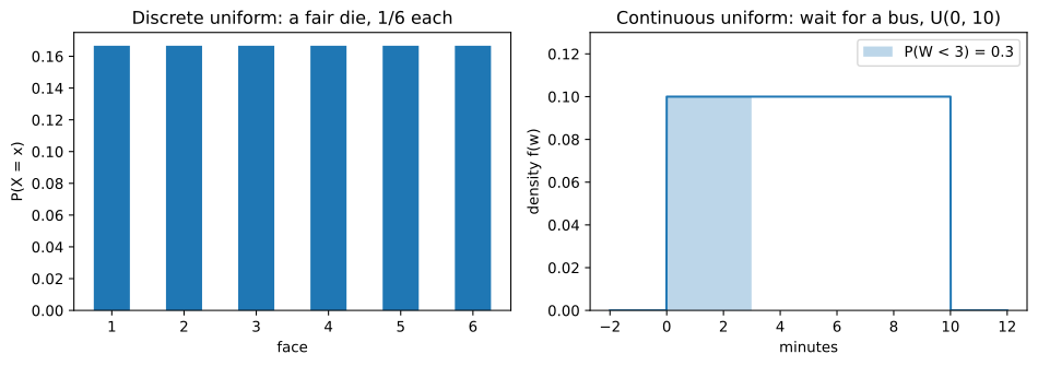
The uniform distribution is the probability distribution in which every value in a range is equally likely: each face of a fair die in the discrete case, every point between a and b in the continuous case.
Last updated: 07 Oct, 2026 · SciPy 1.18
The fair die of Probability basics already had a uniform distribution: six faces at 1/6 each. The continuous version describes a wait or a position when nothing favours one value over another, and it is the starting point of every computer simulation.
Rolling a fair die: the discrete uniform
A discrete uniform variable takes n whole-number values, each with probability 1/n. For values a, a + 1, …, b, with n = b − a + 1:
For a die, a = 1, b = 6 and n = 6: the mean is 3.5 and the variance (36 − 1)/12 = 35/12 ≈ 2.9167, the same values found in the random variables lesson.
Waiting for a bus: the continuous uniform
A bus comes every 10 minutes and you arrive at a random moment. Your wait W is equally likely to be anywhere from 0 to 10 minutes: W ~ U(0, 10). The density is flat at height 1/(b − a), so that the area under it is 1:
For the bus, f(x) = 1/10 = 0.1. A probability is the area of a rectangle: P(W < 3) = 3 × 0.1 = 0.3, and P(2 < W < 7) = 5 × 0.1 = 0.5. The mean wait is 5 minutes and the variance 100/12 ≈ 8.33, a standard deviation of about 2.89 minutes.
Computing uniform probabilities in scipy
scipy describes U(a, b) with loc = a and scale = b − a, not with a and b. stats.uniform(2, 7) is therefore U(2, 9), and randint(1, 7) leaves out its upper end 7. The last lines show the difference.
import numpy as np
from scipy import stats

die = stats.randint(1, 7)                       # 1, 2, ..., 6
print("die: P(X = 4) =", round(die.pmf(4), 4), " mean", die.mean(), " var", round(die.var(), 4))

wait = stats.uniform(loc=0, scale=10)           # U(0, 10): loc = a, scale = b - a
print("bus: f(4) =", wait.pdf(4), " P(W < 3) =", wait.cdf(3), " P(2 < W < 7) =", round(wait.cdf(7) - wait.cdf(2), 4))
print("mean", wait.mean(), " var", round(wait.var(), 4), " sd", round(wait.std(), 4))

rng = np.random.default_rng(42)
waits = rng.uniform(0, 10, size=100_000)        # numpy takes low and high
print("100,000 waits: mean", round(waits.mean(), 3), " share under 3 min", round(np.mean(waits < 3), 4))

print("stats.uniform(2, 7) covers", [float(v) for v in stats.uniform(2, 7).support()], "  mean", stats.uniform(2, 7).mean())
print("U(2, 7) is stats.uniform(loc=2, scale=5):", [float(v) for v in stats.uniform(loc=2, scale=5).support()], " mean", stats.uniform(loc=2, scale=5).mean())die: P(X = 4) = 0.1667 mean 3.5 var 2.9167 bus: f(4) = 0.1 P(W < 3) = 0.3 P(2 < W < 7) = 0.5 mean 5.0 var 8.3333 sd 2.8868 100,000 waits: mean 5.006 share under 3 min 0.2994 stats.uniform(2, 7) covers [2.0, 9.0] mean 5.5 U(2, 7) is stats.uniform(loc=2, scale=5): [2.0, 7.0] mean 4.5
Plotting the two uniform distributions
import numpy as np
import matplotlib.pyplot as plt
from scipy import stats

fig, ax = plt.subplots(1, 2, figsize=(10, 3.6))
x = np.arange(1, 7)
ax[0].bar(x, stats.randint(1, 7).pmf(x), width=0.5)
ax[0].set_title("Discrete uniform: a fair die, 1/6 each")
ax[0].set_xlabel("face")
ax[0].set_ylabel("P(X = x)")

w = np.linspace(-2, 12, 1401)
f = stats.uniform(0, 10).pdf(w)
ax[1].plot(w, f)
ax[1].fill_between(w, f, where=w < 3, alpha=0.3, label="P(W < 3) = 0.3")
ax[1].set_title("Continuous uniform: wait for a bus, U(0, 10)")
ax[1].set_xlabel("minutes")
ax[1].set_ylabel("density f(w)")
ax[1].set_ylim(0, 0.13)
ax[1].legend(loc="upper right")
fig.tight_layout()
plt.show()
print("shaded area P(W < 3) =", stats.uniform(0, 10).cdf(3), " total area =", stats.uniform(0, 10).cdf(10))shaded area P(W < 3) = 0.3 total area = 1.0
What the uniform numbers show
- The die has P(X = 4) = 0.1667, mean 3.5 and variance 2.9167, from the discrete formulas.
- The bus density is 0.1 everywhere in [0, 10]; P(W < 3) = 0.3 and P(2 < W < 7) = 0.5 are rectangle areas.
- The mean wait is 5 minutes with variance 8.3333 and SD 2.8868, matching (b − a)²/12.
- The simulation agrees: 100,000 waits average 5.006 minutes and 0.2994 of them are under 3 minutes.
stats.uniform(2, 7)runs from 2 to 9 with mean 5.5; U(2, 7) needsloc=2, scale=5and has mean 4.5.
Discrete vs continuous uniform
| Discrete uniform | Continuous uniform | |
|---|---|---|
| Values | n whole numbers a, …, b | Every real number in [a, b] |
| Probability of one value | 1/n | 0 (use areas) |
| Mean | (a + b)/2 | (a + b)/2 |
| Variance | (n² − 1)/12 | (b − a)²/12 |
| Example | A fair die | A bus wait |
| scipy | stats.randint(a, b + 1) | stats.uniform(loc=a, scale=b − a) |
Where you use the uniform distribution
- Simulation: random number generators produce uniform values first, and other distributions are built from them.
- Random search: trying hyperparameter values drawn uniformly from a range.
- Rounding and timing: a rounding error, or the time to the next bus on a fixed timetable, is uniform when nothing favours one value.
stats.uniform. Its arguments are loc and scale, so stats.uniform(2, 7) silently means U(2, 9); write loc=a, scale=b - a.Related
- Previous: Poisson distribution
- Next: Log-normal distribution
- A bus every 15 minutes: build
stats.uniform(loc=0, scale=15). What are the mean wait and P(W > 10)? - Check the die's variance with the formula
(6 ** 2 - 1) / 12. - Draw a histogram of
waitswithplt.hist(waits, bins=20). Are the bars about the same height?
Every expert started right here.