
Arbitrary value imputation
Arbitrary value imputation fills the gaps with a number you pick yourself, such as 0 or 100, chosen to sit outside the column's ordinary range so that the filled rows stay recognisable.
Last updated: 12 Oct, 2026 · pandas 3.0
End of distribution imputation computed its fill value from the column. This one is chosen by hand, which makes it the simplest technique here and the one with the most ways to go wrong.
Syntax: Series.fillna(value) with a literal. The whole technique is the choice of that literal, and there are three rules for it: the value must not occur in the data, it should sit at one end of the range, and it is chosen per column, not shared.
df['Age_zero'] = df['Age'].fillna(0)        # below every real age
df['Age_hundred'] = df['Age'].fillna(100)   # above every real age
df['Score'] = df['Score'].fillna(-999)      # a value no score can take
Loading the Titanic data
The Titanic table is 891 passengers. Age is missing for 177 of them, Cabin for 687 and Embarked for 2, which makes it the right table to learn these techniques on. It loads from its GitHub URL, so there is nothing to download. Run this block first, then the example under it.
import pandas as pd
import matplotlib
matplotlib.use('svg')
import matplotlib.pyplot as plt

url = ("https://raw.githubusercontent.com/krishnaik06/"
       "Feature-Engineering-Live-sessions/master/titanic.csv")
df = pd.read_csv(url, usecols=['Survived', 'Age', 'Fare'])
Filling with 0 and with 100
Age runs from 0.42 to 80.0, so 0 sits below everything and 100 above everything. Both are outside the data and neither occurs in it, which is what the technique asks for. describe() on the three versions shows what each choice costs.
print("observed range:", df['Age'].min(), "to", df['Age'].max())
df['Age_zero'] = df['Age'].fillna(0)
df['Age_hundred'] = df['Age'].fillna(100)
print(df[['Age', 'Age_zero', 'Age_hundred']].describe().round(4).to_string())observed range: 0.42 to 80.0
Age Age_zero Age_hundred
count 714.0000 891.0000 891.0000
mean 29.6991 23.7993 43.6646
std 14.5265 17.5961 30.9304
min 0.4200 0.0000 0.4200
25% 20.1250 6.0000 22.0000
50% 28.0000 24.0000 32.0000
75% 38.0000 35.0000 54.0000
max 80.0000 80.0000 100.0000- The mean moves in opposite directions. 29.6991 becomes 23.7993 with zeros and 43.6646 with hundreds, from the same data.
- The standard deviation rises either way. 14.5265 becomes 17.5961 and 30.9304, because both fills push 177 rows away from the centre.
- The quartiles move too. The median falls to 24.0 with zeros and rises to 32.0 with hundreds, so every summary of this column now depends on a number somebody chose.
- Neither version is wrong. They answer different questions, and the model only knows what it is given.
Seeing both spikes
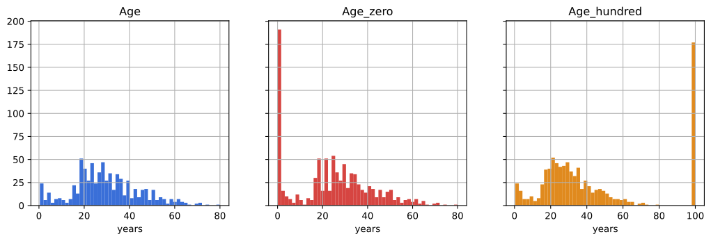
The histograms make the choice concrete: the same hump with a bar of 177 rows bolted on at one end or the other.
df['Age_zero'] = df['Age'].fillna(0)
df['Age_hundred'] = df['Age'].fillna(100)
print("rows sitting at the fill value, zero:", int((df['Age_zero'] == 0).sum()))
print("rows sitting at the fill value, hundred:",
      int((df['Age_hundred'] == 100).sum()))

fig, axes = plt.subplots(1, 3, figsize=(13, 3.6), sharey=True)
for ax, col, colour in zip(axes, ['Age', 'Age_zero', 'Age_hundred'],
                           ['#3a6fd8', '#d64541', '#e08a1e']):
    df[col].hist(bins=50, ax=ax, color=colour)
    ax.set_title(col)
    ax.set_xlabel('years')
fig.savefig('chart.svg')rows sitting at the fill value, zero: 177 rows sitting at the fill value, hundred: 177
Choosing the value
- It must not occur in the data. Filling an age with 0 is safe here because no passenger is recorded as 0; the youngest is 0.42. On a column of counts, 0 is a real value and the fill would be invisible.
- It should sit at one end of the range. A fill in the middle hides among real values and nothing downstream can separate it.
- -999 is the common choice for a column that is never negative, for the same reason, and it is as arbitrary as any other.
- Pick it per column. 100 is far out for an age and ordinary for a fare.
Arbitrary vs end of distribution imputation
| Arbitrary value | End of distribution | |
|---|---|---|
| Where the value comes from | you choose it | mean plus three standard deviations |
| Depends on the data | no | yes, it is recomputed per column |
| Works on a train and test split | the same literal both sides | the value must be learned on train and reused on test |
| Risk | picking a value that occurs in the data | a fence that the data never reaches |
| Readable afterwards | yes, 0 and -999 are obvious | less so, 73.2786 looks like data |
Where an arbitrary value is used
- Competition style tabular work. Fast, explicit, and a tree model separates the fill value in one split.
- Codes that already have a sentinel. Some sources write -1 or 9999 for unknown, and matching their convention keeps the column consistent.
- A column you plan to bin. The fill value becomes its own bin, which is the categorical answer in Missing as its own category.
Related
- Previous: End of distribution imputation
- Next: Frequent category imputation
- See also: Mean and median imputation
- Reference: SimpleImputer with
strategy='constant'
- Fill with 29.0, a value that does occur in the data, and try to find the filled rows afterwards.
- Compare
df['Age_zero'].corr(df['Survived'])with the correlation of the median filled column. - Fill
Farewith -999 and read what it does todescribe().
Slow is fine. Stopping is the only problem.