
Why features are scaled
Feature scaling is a preparation step that puts every numeric column on a comparable range, so that no column counts for more only because its numbers are larger.
Last updated: 12 Oct, 2026 · pandas 3.0 · scikit-learn 1.9 · scipy 1.18
Handling an unknown category finished turning text into numbers. Those numbers now sit in the same table as Age, Fare and Price, and their ranges do not match: a one hot column holds 0 or 1 while Fare runs from 0 to 512. Several model families read that difference as importance, and the arithmetic that makes them do it is short enough to work out by hand.
Measuring the gap between two rows
A model such as k nearest neighbours decides which rows are alike by the straight line distance between them. For two features that distance is the square root of the squared difference in each one, which is the Euclidean distance the video writes on the board.
The two points from the video
The board holds two rows, (24, 54) and (30, 70). The first feature differs by 6 and the second by 16. Squaring is what turns that into a lopsided contribution.
p = np.array([24.0, 54.0])    # the first row: feature 1 = 24, feature 2 = 54
q = np.array([30.0, 70.0])    # the second row
gaps = (p - q) ** 2           # the squared difference in each feature
Working out the two point distance
import numpy as np

p = np.array([24.0, 54.0])    # the first row: feature 1 = 24, feature 2 = 54
q = np.array([30.0, 70.0])    # the second row
gaps = (p - q) ** 2           # the squared difference in each feature

print("squared gaps:", gaps.tolist())
print("distance    :", round(float(np.sqrt(gaps.sum())), 4))
print("share of the distance from feature 2:", f"{gaps[1] / gaps.sum():.1%}")squared gaps: [36.0, 256.0] distance : 17.088 share of the distance from feature 2: 87.7%
- squared gaps: [36.0, 256.0] is the arithmetic: a gap of 6 becomes 36, a gap of 16 becomes 256.
- distance 17.088 is the square root of 36 + 256.
- 87.7% of that distance comes from the second feature alone, although the two features moved by 6 and 16. Squaring widens every head start.
What one wide column does to a real dataset
Titanic has the same shape of problem at full size. Age runs from 0.42 to 80 and Fare from 0 to 512.33, so Fare's gaps are the only ones a distance ever notices. Dividing each column by its own maximum is the cheapest possible fix, and it is the one the video names for image pixels, where every value is divided by 255.
import pandas as pd

URL = "https://raw.githubusercontent.com/krishnaik06/Feature-Engineering-Live-sessions/master/titanic.csv"
df = pd.read_csv(URL, usecols=['Age', 'Fare'])
df['Age'] = df['Age'].fillna(df['Age'].median()) # 177 missing ages, filled with 28.0def shares(frame, label):
sq = (frame.loc[0] - frame.loc[1]) ** 2 # squared gap, column by column
print(f"{label:24s} distance {np.sqrt(sq.sum()):7.3f}"
f" Age {sq['Age'] / sq.sum():6.1%} Fare {sq['Fare'] / sq.sum():6.1%}")Comparing the first two passengers before and after
import numpy as np
import matplotlib.pyplot as plt
def shares(frame, label):
    sq = (frame.loc[0] - frame.loc[1]) ** 2       # squared gap, column by column
    print(f"{label:24s} distance {np.sqrt(sq.sum()):7.3f}"
          f"   Age {sq['Age'] / sq.sum():6.1%}   Fare {sq['Fare'] / sq.sum():6.1%}")
scaled = df / df.max() # every column now runs from 0 to 1
shares(df, "raw values")
shares(scaled, "divided by the maximum")
fig, ax = plt.subplots(1, 2, figsize=(9, 3.2))
for a, frame, title in [(ax[0], df, "raw values"), (ax[1], scaled, "divided by the maximum")]:
for y, col, colour in [(1, "Age", "#3a6fd8"), (0, "Fare", "#d8733a")]:
a.hlines(y, frame[col].min(), frame[col].max(), color=colour, lw=9)
a.annotate(f"{frame[col].min():.1f} to {frame[col].max():.1f}",
(frame[col].max(), y), xytext=(6, 0), textcoords="offset points",
va="center", fontsize=9)
a.set_yticks([0, 1]); a.set_yticklabels(["Fare", "Age"])
a.set_ylim(-0.6, 1.6); a.set_title(title); a.margins(x=0.3)
fig.tight_layout()raw values distance 66.002 Age 5.9% Fare 94.1% divided by the maximum distance 0.236 Age 71.9% Fare 28.1%
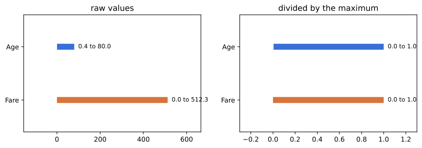
Reading the two distance lines
- raw values put 94.1% of the squared distance on Fare. Age contributes 5.9%, so a neighbour search on this table is close to a neighbour search on Fare alone.
- divided by the maximum moves the split to 71.9% Age and 28.1% Fare. Neither column is now ignored because of its units.
- The distance itself shrinks from 66.0 to 0.236. The number means nothing on its own; what matters is which column it is made of.
What the gap does to a model being trained
A model trained by gradient descent walks downhill on a surface built from the columns. When one column is wide and another is narrow, that surface is a long thin valley, and each step crosses it rather than running along it. Putting the columns on one scale makes the surface round, and the same walk is shorter.
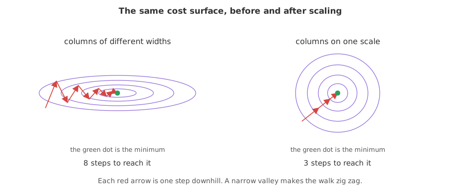
Raw columns compared with scaled columns
| Raw columns | Scaled columns | |
|---|---|---|
| Range | whatever the units give, 0 to 512 for Fare | a known range, such as 0 to 1 |
| Distance | decided by the widest column | every column can contribute |
| Gradient descent | long thin valleys, small steps, many rounds | rounder surface, fewer rounds |
| Tree splits | unchanged | unchanged |
| Cost | none | one fitted object to carry to prediction time |
Where scaling changes the answer
- Distance based models. k nearest neighbours, k means and hierarchical clustering all rank rows by Euclidean distance, so the widest column decides the ranking.
- Models trained by gradient descent. Linear regression, logistic regression and every neural network walk downhill on a cost surface. Columns of different widths stretch that surface into a narrow valley, and the walk takes more rounds.
- Image inputs. Pixels arrive as 0 to 255 and are divided by 255 before training, which is exactly the division run above.
Related
- Previous: Handling an unknown category
- Next: Which algorithms need scaling
- See also: Standardisation
- Reference: Preprocessing data in the scikit-learn docs
- Change the board's second point from
(30, 70)to(30, 55)and read the share again. The second feature stops dominating because its gap is now 1. - Divide only
Fareby its maximum and leaveAgealone. The share flips the other way, which shows that half a fix is its own problem. - Swap
df.max()fordf.mean(). The ranges no longer land in 0 to 1, and the shares move again.
Every expert started right here.