
Box-Cox and Yeo-Johnson
Box-Cox and Yeo-Johnson are power transformations that search for the exponent which makes a column as close to normal as possible, instead of asking you to guess it.
Last updated: 12 Oct, 2026 · pandas 3.0 · scikit-learn 1.9 · scipy 1.18
Log, reciprocal and square root transformations ended with a hand picked exponent of 1/1.2 and a note that a better one exists. These two transformations find it. The difference between them is one line of their definition, and that line decides which columns each can handle.
The Box-Cox formula
Box-Cox is one family of curves controlled by a single number, lambda. Lambda of 1 leaves the shape alone, 0.5 gives the square root, 0 gives the logarithm and −1 the reciprocal, each up to a shift and a rescale that leaves the shape where it was. The search tries every lambda between −5 and 5 and keeps the one whose result is closest to normal.
Syntax: scipy.stats.boxcox returns the transformed values and the lambda it chose.
import scipy.stats as stats

transformed, lam = stats.boxcox(values)   # values must all be greater than 0
Finding the best lambda for Age
Age has no zeros and no negative values once the missing rows are filled, so Box-Cox applies directly. The lambda it returns can be compared with the 1/1.2 exponent picked by hand.
import pandas as pd

URL = "https://raw.githubusercontent.com/krishnaik06/Feature-Engineering-Live-sessions/master/titanic.csv"
df = pd.read_csv(URL, usecols=['Age', 'Fare'])
df['Age'] = df['Age'].fillna(df['Age'].median()) # 177 missing ages, filled with 28.0import numpy as np
import scipy.stats as stats
transformed, lam = stats.boxcox(df['Age'])
(_, _), (_, _, r) = stats.probplot(transformed, dist='norm')
(_, _), (_, _, r_raw) = stats.probplot(np.asarray(df['Age']), dist='norm')
print("lambda chosen :", lam)
print("as an exponent : x ** %.4f" % lam)
print("R² before :", round(r_raw ** 2, 4))
print("R² after :", round(r ** 2, 4))
print("skew after :", round(float(stats.skew(transformed)), 4))lambda chosen : 0.796453194094064 as an exponent : x ** 0.7965 R² before : 0.9542 R² after : 0.9602 skew after : 0.0604
- Lambda is 0.796453194094064. Read as an exponent that is x to the power 0.7965, which sits between the square root at 0.5 and no transformation at 1.
- The hand picked 1/1.2 was 0.8333, so the search landed on the same part of the family without being told: R² 0.9602 against 0.9604, a tie. The value of the search is that it needed no guessing and no five panel chart. Box-Cox also subtracts 1 and divides by lambda, which shifts and rescales the result, so the two are not the same numbers.
- Skew drops to 0.0604, the closest to symmetric of anything tried on this column.
The error Box-Cox gives on a column with zeros
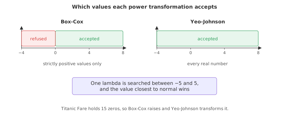
Fare is the column that needs the most help, and it is the one Box-Cox refuses. The formula contains y raised to a power and a logarithm, neither of which is defined at 0 or below, so scipy stops rather than returning nonsense.
import pandas as pd
import scipy.stats as stats

URL = "https://raw.githubusercontent.com/krishnaik06/Feature-Engineering-Live-sessions/master/titanic.csv"
df = pd.read_csv(URL, usecols=['Age', 'Fare'])

print("smallest fare:", df["Fare"].min())
stats.boxcox(df['Fare'])smallest fare: 0.0
Traceback (most recent call last):
File "main.py", line 8, in <module>
stats.boxcox(df['Fare'])
ValueError: Data must be positive.The usual answer in 2020 was to add 1 to the column and transform df['Fare'] + 1. That works, and it is a decision taken for the solver's benefit rather than the data's: the shift changes the lambda that is chosen, and it has to be repeated identically on every future row. A column whose values can be negative, such as a temperature or a profit and loss figure, cannot be rescued that way at all.
Yeo-Johnson, which accepts any value
Yeo-Johnson is the same idea with the formula extended so that negative and zero values have their own branch. It needs no shift, no constant and no decision from you, and on a strictly positive column it gives the same answer Box-Cox would.
Syntax: scikit-learn's PowerTransformer offers both methods and, unlike scipy, works on a whole frame and remembers its lambdas for new data.
from sklearn.preprocessing import PowerTransformer

pt = PowerTransformer(method='yeo-johnson')   # the default; 'box-cox' is the other
out = pt.fit_transform(frame)                 # standardize=True, so the output has mean 0
Transforming the fares that Box-Cox refused
import numpy as np
import matplotlib.pyplot as plt
import scipy.stats as stats
from sklearn.preprocessing import PowerTransformer

pt = PowerTransformer(method='yeo-johnson').set_output(transform='pandas')
out = pt.fit_transform(df[['Fare']])

fig, ax = plt.subplots(1, 2, figsize=(9, 3.4))
for a, values, name in [(ax[0], df['Fare'], 'Fare'), (ax[1], out['Fare'], 'Yeo-Johnson(Fare)')]:
    (osm, osr), (slope, intercept, r) = stats.probplot(np.asarray(values), dist='norm')
    a.plot(osm, slope * osm + intercept, color='#c23b22', lw=1.1, ls='--')
    a.plot(osm, osr, color='#3a6fd8', lw=1.6)
    a.set_title(f'{name}  R²={r ** 2:.4f}', fontsize=10)
    a.set_xlabel('normal quantiles')
    print(f"{name:20s} skew {stats.skew(values):7.3f}   R² {r ** 2:.4f}")
fig.tight_layout()
print("lambda chosen:", pt.lambdas_[0])
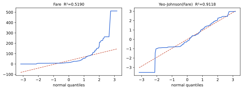
print("mean and std after:", round(float(out["Fare"].mean()), 10), round(float(out["Fare"].std(ddof=0)), 6))Fare skew 4.779 R² 0.5190 Yeo-Johnson(Fare) skew -0.040 R² 0.9118 lambda chosen: -0.09778703637848858 mean and std after: -0.0 1.0
Reading the Yeo-Johnson result
- Lambda is −0.0978, close to 0, which is the logarithm end of the family. The search reached the same conclusion as the log1p choice in the previous lesson, without being told.
- R² rises from 0.5190 to 0.9118 and skew falls from 4.779 to −0.04. The 15 zero fares went through untouched.
- The mean prints as −0.0 and the standard deviation as 1.
PowerTransformerstandardises after transforming by default, so no separateStandardScalerstep is needed. - The lambdas are stored on the fitted object, so the same transformation can be applied to new rows with
pt.transform(...). scipy's function gives you a number and leaves the bookkeeping to you.
Box-Cox compared with Yeo-Johnson
| Box-Cox | Yeo-Johnson | |
|---|---|---|
| Accepts | strictly positive values only | any real value, zero and negative included |
| On a column with a 0 | raises ValueError: Data must be positive | transforms it |
| Workaround needed | shift the column, and repeat the shift on new data | none |
| In scipy | stats.boxcox | stats.yeojohnson |
| In scikit-learn | PowerTransformer(method='box-cox') | PowerTransformer(), the default |
| On a strictly positive column | the same answer | the same answer |
Picking a scaler or a transformation for a column
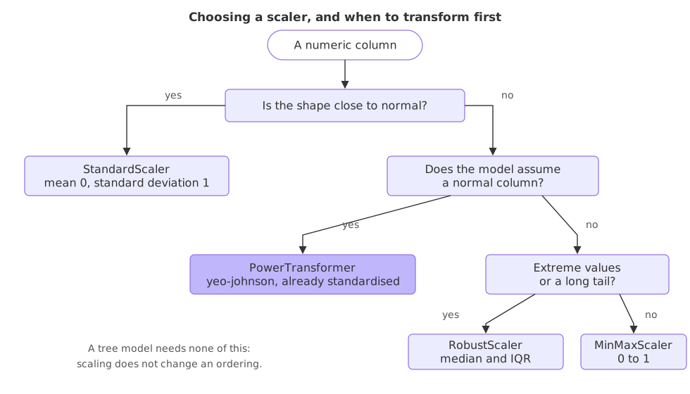
With all four tools in hand the choice follows from two questions about the column and one about the model.
Where a power transformation is used
- As the default when a column must be made normal. Yeo-Johnson needs no inspection of the column's minimum, which makes it the safe choice inside a pipeline fitted on data you have not looked at.
- On a regression target, through
TransformedTargetRegressor, which applies the transformation to the target and undoes it on every prediction. - On columns that can be negative, such as temperatures, profit and loss or any difference between two measurements, where Box-Cox cannot be used at all.
transform on the test rows, never fit_transform twice. And a column with a single NaN still in it makes scipy.stats.boxcox return a lambda of nan with no warning, so fill first.Related
- Previous: Log, reciprocal and square root transformations
- Next: Splitting a date into columns
- See also: Split first, then fit
- Reference: PowerTransformer in the scikit-learn docs
- Call
PowerTransformer(method='box-cox')on the Fare frame. The message differs from scipy's and says the same thing. - Pass
standardize=Falseand look at the mean again. The shape is the same; only the axis changes. - Transform
df[['Age', 'Fare']]in one call and printpt.lambdas_. One lambda is learned per column, not one for the frame.
You understood something today that you didn't yesterday.