
Frequent category imputation
Frequent category imputation fills the gaps in a text column with its mode, the category that appears most often, which completes the column at the cost of making that category more common than it is.
Last updated: 12 Oct, 2026 · pandas 3.0
Arbitrary value imputation finished the numeric techniques. A text column has no mean and no median, so the only summary available is the most frequent value, and whether it can be used depends on how much of the column is missing.
The clip works on an online retail table whose two product category columns hold a small set of repeated codes. A column like that is discrete rather than continuous, which is why its gaps are filled with the most frequent value and not with an average: an average would invent a code that no product has. The examples here run the same technique on the house price table, which loads from its GitHub URL, and add the measurement of what the fill costs.
Syntax: Series.mode() returns a Series, because a column can have two equally frequent values, so the mode itself is mode()[0]. value_counts().index[0] gives the same answer.
df['GarageType'].mode()          # a Series, not a value
df['GarageType'].mode()[0]       # the most frequent category
df['GarageType'].value_counts().index[0]        # the same thing
df['GarageType'] = df['GarageType'].fillna(df['GarageType'].mode()[0])
Loading the house price data
These examples use the house price table, 1,460 houses, and four of its columns: three text columns with missing values and the sale price to measure the damage against. Run this block first, then the example under it.
import pandas as pd
import matplotlib
matplotlib.use('svg')
import matplotlib.pyplot as plt

url = ("https://raw.githubusercontent.com/krishnaik06/"
       "Advanced-House-Price-Prediction-/master/train.csv")
df = pd.read_csv(url, usecols=['BsmtQual', 'FireplaceQu',
                               'GarageType', 'SalePrice'])
How much of each column is missing, and what its mode is
The share missing is the number that decides whether this technique can be used at all, so it comes first. isnull().mean() gives it, and the two ways of reading the mode agree.
print(df.isnull().sum().to_string())
print()
print("share missing, in percent:")
print((df.isnull().mean() * 100).round(4).sort_values().to_string())
print()
for col in ['BsmtQual', 'GarageType', 'FireplaceQu']:
    print(f"{col:12s} mode {df[col].mode()[0]:8s}"
f" value_counts().index[0] {df[col].value_counts().index[0]}")BsmtQual 37 FireplaceQu 690 GarageType 81 SalePrice 0 share missing, in percent: SalePrice 0.0000 BsmtQual 2.5342 GarageType 5.5479 FireplaceQu 47.2603 BsmtQual mode TA value_counts().index[0] TA GarageType mode Attchd value_counts().index[0] Attchd FireplaceQu mode Gd value_counts().index[0] Gd
- BsmtQual is missing 2.5342 percent and GarageType 5.5479 percent. Both are small enough for a mode fill to change very little.
- FireplaceQu is missing 47.2603 percent. Nearly half the column is absent, which is a different problem.
- The modes are TA, Attchd and Gd. Both ways of finding them return the same value, and
mode()needs its[0]because it returns a Series.
As a rule of thumb, frequent category imputation is for columns missing a few percent, and it stops being reasonable somewhere around 40 percent missing. Past that point the fill is no longer a repair; it is most of the column.
Filling the two columns that qualify
A loop over the columns keeps the code short. Assigning the result back is what makes the fill stick: an in-place fill reached through a column reference does nothing, which Copy-on-write and chained assignment shows in full.
for col in ['BsmtQual', 'GarageType']:
    df[col] = df[col].fillna(df[col].mode()[0])
print("nulls left:")
print(df[['BsmtQual', 'GarageType']].isnull().sum().to_string())
print()
print("GarageType after the fill:")
print(df['GarageType'].value_counts().to_string())nulls left: BsmtQual 0 GarageType 0 GarageType after the fill: GarageType Attchd 951 Detchd 387 BuiltIn 88 Basment 19 CarPort 9 2Types 6
Attchd rises from 870 houses to 951, which is 81 rows moved into the largest category. On a column that was 94 percent complete, that is a small distortion and a complete column in return.
What the same fill does to a column that is half empty
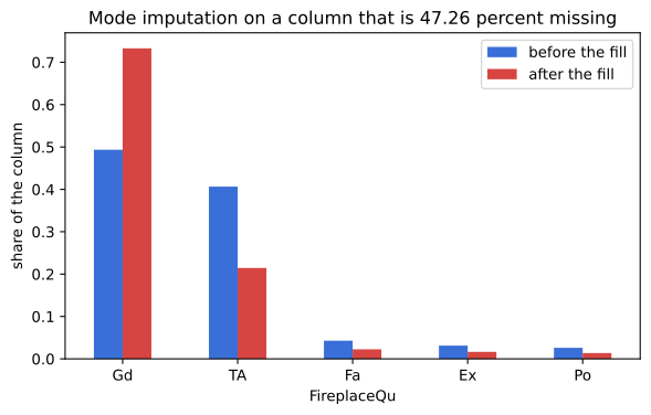
FireplaceQu is the warning. Its mode, Gd, holds 49.35 percent of the recorded values. Filling 690 gaps with it pushes that share to 73.29 percent, so the category that described half the fireplaces now describes three quarters of the houses.
before = df['FireplaceQu'].value_counts(normalize=True).round(4)
after = (df['FireplaceQu'].fillna(df['FireplaceQu'].mode()[0])
         .value_counts(normalize=True).round(4))
shares = pd.DataFrame({'before the fill': before, 'after the fill': after})
print(shares.to_string())

fig, ax = plt.subplots(figsize=(7, 4))
shares.plot.bar(ax=ax, color=['#3a6fd8', '#d64541'], rot=0)
ax.set_ylabel('share of the column')
ax.set_title('Mode imputation on a column that is 47.26 percent missing')
fig.savefig('chart.svg')before the fill after the fill FireplaceQu Gd 0.4935 0.7329 TA 0.4065 0.2144 Fa 0.0429 0.0226 Ex 0.0312 0.0164 Po 0.0260 0.0137
Measuring the damage against the target
A share moving is abstract. The same fill seen against the sale price is not: the houses with no fireplace are cheaper than the houses with a good one, and pouring them into the Gd category drags that category's median price down with them.
filled = df['FireplaceQu'].fillna(df['FireplaceQu'].mode()[0])
medians = pd.DataFrame({
    'before the fill': df.groupby('FireplaceQu')['SalePrice'].median(),
    'after the fill': df.assign(f=filled).groupby('f')['SalePrice'].median()})
print(medians.round(0).to_string())

fig, ax = plt.subplots(figsize=(7, 4))
medians.plot.bar(ax=ax, color=['#3a6fd8', '#d64541'], rot=0)
ax.set_ylabel('median SalePrice')
ax.set_title('What the fill does to the price of each fireplace grade')
fig.savefig('chart.svg')before the fill after the fill Ex 314250.0 314250.0 Fa 158000.0 158000.0 Gd 206950.0 149525.0 Po 131500.0 131500.0 TA 187500.0 187500.0
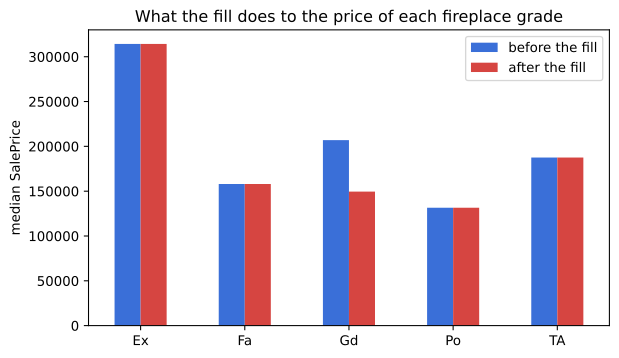
- Gd falls from 206,950 to 149,525. Every other grade is untouched, because no rows were added to them.
- The ranking breaks. Before the fill Gd was the second most expensive grade; after it, Gd is cheaper than TA and Fa, which is the opposite of what the grade means.
- Any encoder that uses the target now learns the wrong order, which is what Target guided ordinal encoding depends on.
- No warning was printed. The column is complete and the damage is only visible when you look for it.
The honest treatment of a column like this is to keep the absence instead of hiding it, which is Missing as its own category.
Mode fill vs a category of its own
| Frequent category imputation | Missing as its own category | |
|---|---|---|
| Fill value | the most frequent category | a new label such as Missing |
| Number of categories after | unchanged | one more |
| Use when the share missing is | small, a few percent | any size, and meaningful |
| Effect on the modal category | it grows | none |
| Keeps the missingness signal | no | yes |
Where the mode is the right fill
- A text column missing a handful of rows. Two missing ports of embarkation out of 891: the mode is the fastest honest answer.
- A discrete numeric code. A product category or a rating level repeats a small set of values, so the mode works where a mean would invent a code.
- Inside a pipeline.
SimpleImputer(strategy='most_frequent')learns the mode on the training rows only, which is what SimpleImputer in scikit-learn is for.
mode() returns a Series because two categories can tie, and fillna(df[c].mode()) without the [0] fills with a Series, which aligns on the index and leaves most of the gaps in place. Always take [0], and when the counts tie, say which value you took.Related
- Previous: Arbitrary value imputation
- Next: Missing as its own category
- See also: Counting categories with value_counts
- Reference: Series.mode in the pandas docs
- Fill
FireplaceQuwith its mode and comparedf.groupby('FireplaceQu')['SalePrice'].size()before and after. - Write
df['BsmtQual'].fillna(df['BsmtQual'].mode())without the[0]and count the nulls left. - Find a column in the full house price table whose two most frequent categories are close in count, and decide which one you would fill with.
This is what real progress feels like.