
Treating outliers by capping or dropping
Capping replaces every value past a boundary with the boundary itself, which keeps the row, keeps its other columns and removes the pull the far value had.
Last updated: 12 Oct, 2026 · pandas 3.0 · scikit-learn 1.9
The IQR fence produced a number: a fence at 65.63 with 116 fares past it. This lesson is about what to do with those 116 rows, and about why the answer is almost never to delete them.
Syntax: Series.clip pulls every value back inside a boundary in one call.
capped = s.clip(upper=65.63)          # anything above becomes 65.63
capped = s.clip(lower=0, upper=65.63)  # both ends at once
Capping the Fare column at its fence
The boundary comes from the fence
The cap is not a round number picked by hand. It is the fence the previous lesson computed, so the same rule that flagged the rows also decides where they land.
q1, q3 = fare.quantile(0.25), fare.quantile(0.75)
fence = q3 + 1.5 * (q3 - q1)
Writing the capped column back
clip returns a new Series, so the result has to be assigned. Under pandas 3 a write through df['Fare'][mask] = fence lands on a throwaway copy and changes nothing, which Copy-on-write and chained assignment shows in full.
df["Fare"] = df["Fare"].clip(upper=fence) # assign it backWhat capping changed, and what it did not
import matplotlib
matplotlib.use("svg")
import matplotlib.pyplot as plt
import pandas as pd

URL = ("https://raw.githubusercontent.com/krishnaik06/Feature-Engineering-Live-sessions/"
       "master/titanic.csv")
fare = pd.read_csv(URL)["Fare"]

q1, q3 = fare.quantile(0.25), fare.quantile(0.75)
fence = q3 + 1.5 * (q3 - q1)
capped = fare.clip(upper=fence)

print("fence:", fence)
print("values changed:", int((fare > fence).sum()), "of", len(fare))
print("rows lost:", len(fare) - len(capped))
print("max   before:", fare.max(), " after:", capped.max())
print("mean  before:", round(fare.mean(), 4), " after:", round(capped.mean(), 4))
print("median before:", fare.median(), " after:", capped.median())

fig, ax = plt.subplots(figsize=(7, 2.6))
ax.boxplot([fare, capped], orientation="horizontal", widths=0.5)
ax.set_yticklabels(["before", "after"])
ax.set_xlabel("Fare")
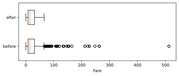
fig.savefig("chart.svg")fence: 65.6344 values changed: 116 of 891 rows lost: 0 max before: 512.3292 after: 65.6344 mean before: 32.2042 after: 24.0468 median before: 14.4542 after: 14.4542
Reading the before and after
- 116 values changed and no rows were lost. Every passenger is still in the frame, with their class, age and port untouched. That is the whole argument for capping over dropping.
- The maximum fell from 512.33 to 65.63. The column now stops at the fence by construction.
- The mean fell from 32.20 to 24.05 and the median did not move. The median was never affected by the tail, so capping could not change it.
- The box plot has no points outside the whiskers. It cannot have any: every value past the fence is now exactly at the fence, and the fence was recomputed on a column whose tail is gone.
The last point is worth holding on to. A capped column always looks clean in a box plot. The chart stops being evidence once you have capped, so record what you capped and at what value rather than reading it back off the picture.
Measuring capping against dropping
Three models on the same two columns and the same test rows: one left alone, one with Fare capped, one with the flagged training rows deleted. The fence is computed from the training half only, which is why it comes out at 66.58 here and not at the 65.63 the whole column gave. A boundary computed from the test rows has read data the model will not have, which Data leakage covers.
import pandas as pd
from sklearn.linear_model import LogisticRegression
from sklearn.metrics import roc_auc_score
from sklearn.model_selection import train_test_split

URL = ("https://raw.githubusercontent.com/krishnaik06/Feature-Engineering-Live-sessions/"
       "master/titanic.csv")
df = pd.read_csv(URL, usecols=["Age", "Fare", "Survived"])
df["Age"] = df["Age"].fillna(df["Age"].median())
X_train, X_test, y_train, y_test = train_test_split(
    df[["Age", "Fare"]], df["Survived"], test_size=0.3, random_state=0)

def auc(a, b, c, d, label):
    model = LogisticRegression(max_iter=1000).fit(a, b)
    print(f"{label:22s} roc_auc {roc_auc_score(d, model.predict_proba(c)[:, 1]):.4f}"
          f"   train rows {len(a)}")

q1, q3 = X_train["Fare"].quantile(0.25), X_train["Fare"].quantile(0.75)
fence = q3 + 1.5 * (q3 - q1)              # from the training half only
print("fence:", round(fence, 4))
auc(X_train, y_train, X_test, y_test, "left as they are")
auc(X_train.assign(Fare=X_train["Fare"].clip(upper=fence)), y_train,
    X_test.assign(Fare=X_test["Fare"].clip(upper=fence)), y_test, "Fare capped")
keep = X_train["Fare"] <= fence
auc(X_train[keep], y_train[keep], X_test, y_test, "outlier rows dropped")
print("rows dropped:", int((~keep).sum()), "of", len(X_train))fence: 66.5812 left as they are roc_auc 0.7263 train rows 623 Fare capped roc_auc 0.7413 train rows 623 outlier rows dropped roc_auc 0.7425 train rows 539 rows dropped: 84 of 623
What the three scores say
- Both treatments beat leaving the column alone. 0.7263 goes to 0.7413 with capping and 0.7425 with dropping. Logistic regression is one of the models the far values were pulling.
- Capping and dropping score within 0.0012 of each other. On this column there is no accuracy argument for deleting rows.
- Dropping cost 84 of 623 training rows. 13% of the data, and every other column in those rows went with it.
- Only one of the two survives prediction time. A capped column can be capped again on new data. A dropped row cannot be dropped from a request the model has been asked to answer, so the model meets rows at prediction time of a kind it never saw in training.
Cap, drop or keep
| What it does | Cost | Use it when | |
|---|---|---|---|
| Cap | pulls the value back to a boundary | the magnitude beyond the boundary is lost | the value is real but its size is distorting the fit |
| Drop the row | removes the row | the whole row goes, and it cannot be done at prediction time | the row is a confirmed error you cannot correct |
| Treat as missing | replaces the value with NaN, then imputes | an invented value takes the place of a real one | the value is impossible, such as an age of 300 |
| Keep it | changes nothing | the model has to tolerate the tail | the model is a tree, or the tail is the thing you are predicting |
| Transform the column | a log or similar shrinks the tail | every value changes, and predictions come back in new units | the column is skewed rather than dirty |
Fraud, failure and churn all live in the tail. In those problems the rows the fence flags are the rows the model exists to find, and the right answer is the last two rows of that table.
Where each choice shows up
- Capping a price column before a linear model. The handful of enormous orders stop setting the slope, and every customer stays in the training set.
- Treating an impossible value as missing. A birth year of 1800 is not a cap candidate; it is a hole, and the missing-value part already has the tools for it.
- Keeping everything and changing model. A gradient boosting model splits on order, so the 512 fare and the 100 fare fall on the same side of every split above 100 and the tail costs nothing.
Related
- Previous: The IQR fence
- Next: Nominal and ordinal features
- See also: Split first, then fit
- Reference: pandas.Series.clip
- Cap at the extreme fence,
q3 + 3 * (q3 - q1), and read the three scores again. - Add
lower=to theclipcall with the lower fence and check that nothing changes, because the minimum fare is 0. - Drop the rows from the test half as well as the training half and watch the score rise for a reason that will not hold in production.
Every expert started right here.