
What imbalance does to a model
Class imbalance is a classification problem in which one class holds almost every row, so a model that never once predicts the rare class still scores high accuracy.
Last updated: 12 Oct, 2026 · pandas 3.0 · scikit-learn 1.9
The features built in Cyclical encoding for hours and weekdays all describe the input columns. This part turns to the target column, and to the case where one of its values is rare: fraud among honest payments, a failed part among good ones, a cancelled policy among renewed ones. The rare value is the one anyone cares about, and it is the one a model quietly learns to ignore.
Syntax: three calls read the result of a classification on an imbalanced target. Accuracy on its own does not.
from sklearn.metrics import confusion_matrix, classification_report

pd.Series(y).value_counts(normalize=True)   # how rare is the rare class
confusion_matrix(y_test, pred)              # the four counts behind any score
classification_report(y_test, pred)         # precision and recall per class
Building a 99 to 1 dataset
Generating the rows with make_classification
make_classification draws a dataset with a target whose class shares you choose. weights=[0.99, 0.01] asks for 99 per cent of the rows in class 0 and 1 per cent in class 1. Every other argument below is set so the result is the same on every machine and can be drawn on a page.
from sklearn.datasets import make_classification

X, y = make_classification(
    n_samples=5000,          # rows
    n_features=2,            # two columns, so the rows can be drawn
    n_informative=2,         # both columns carry signal
    n_redundant=0,           # no column is a combination of others
    n_clusters_per_class=1,  # one blob per class
    weights=[0.99, 0.01],    # 99 per cent class 0, 1 per cent class 1
    flip_y=0,                # no random label flipping
    class_sep=0.5,           # how far apart the two blobs sit
    random_state=0,          # the same 5000 rows every run
)
flip_y=0 matters here. Its default flips a small share of labels at random, which on a 1 per cent class would double the minority by accident. class_sep=0.5 pushes the two blobs close together, which is what a hard real problem looks like.
import pandas as pd

from sklearn.datasets import make_classification

X, y = make_classification(
    n_samples=5000,          # rows
    n_features=2,            # two columns, so the rows can be drawn
    n_informative=2,         # both columns carry signal
    n_redundant=0,           # no column is a combination of others
    n_clusters_per_class=1,  # one blob per class
    weights=[0.99, 0.01],    # 99 per cent class 0, 1 per cent class 1
    flip_y=0,                # no random label flipping
    class_sep=0.5,           # how far apart the two blobs sit
    random_state=0,          # the same 5000 rows every run
)

counts = pd.Series(y).value_counts()
print(counts)
print()
print(counts / len(y))0 4950 1 50 Name: count, dtype: int64 0 0.99 1 0.01 Name: count, dtype: float64
- Class 0 has 4950 rows and class 1 has 50. That is a 99 to 1 split, which is mild next to real fraud data where the rare class can be one row in two thousand.
- The shares print as 0.99 and 0.01 exactly, because
flip_y=0stopped any label from being flipped. - Counting the target is the first thing to do on any classification problem, before a single model is fitted.
Drawing the two classes
With two features the whole dataset fits on one chart, and the shape of the problem is visible at a glance.
import numpy as np
import matplotlib.pyplot as plt

rng = np.random.default_rng(0)          # a readable sample of the majority cloud
majority = X[y == 0]
shown = majority[rng.choice(len(majority), 1500, replace=False)]

plt.figure(figsize=(6, 4.5))
plt.scatter(shown[:, 0], shown[:, 1], s=6, color="#b9bfd0",
            label=f"class 0 (1500 of {len(majority)} drawn)")
plt.scatter(X[y == 1, 0], X[y == 1, 1], s=26, color="#d64541", marker="x",
            label=f"class 1 (all {int((y == 1).sum())})")
plt.xlabel("feature 1")
plt.ylabel("feature 2")
plt.title("4950 rows of class 0, 50 rows of class 1")
plt.legend(loc="upper left")
plt.show()
print("minority rows drawn:", int((y == 1).sum()))minority rows drawn: 50
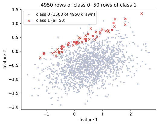
The crosses are not in a corner of their own. They lie along the upper edge of the grey cloud and overlap it, so no straight line separates the two classes cleanly. A model has to choose how much majority territory to give up in order to catch them.
Fitting a model and reading its accuracy
Splitting with stratify
The split comes first, before anything is fitted or counted. train_test_split cuts the rows into a part the model learns from and a part it is scored on, and stratify=y keeps the class shares the same in both halves. Without it a random 30 per cent test set of 50 minority rows can end up with far fewer than 15, and the test score becomes luck. Split first, then fit covers why the order matters for every step in this course, not only for an imbalanced target.
from sklearn.model_selection import train_test_split

X_train, X_test, y_train, y_test = train_test_split(
    X, y, test_size=0.3, random_state=42, stratify=y)
Training a logistic regression
max_iter=1000 raises the iteration budget so the solver converges and prints no warning. No other setting on the model is changed.
from sklearn.linear_model import LogisticRegression

model = LogisticRegression(max_iter=1000).fit(X_train, y_train)
pred = model.predict(X_test)from sklearn.metrics import accuracy_score, confusion_matrix, classification_report
from sklearn.linear_model import LogisticRegression
model = LogisticRegression(max_iter=1000).fit(X_train, y_train)
pred = model.predict(X_test)
print("accuracy:", accuracy_score(y_test, pred))
print("test rows predicted as class 1:", int(pred.sum()))
print()
print(confusion_matrix(y_test, pred))
print()
print(classification_report(y_test, pred, digits=3))accuracy: 0.99
test rows predicted as class 1: 0
[[1485 0]
[ 15 0]]
precision recall f1-score support
0 0.990 1.000 0.995 1485
1 0.000 0.000 0.000 15
accuracy 0.990 1500
macro avg 0.495 0.500 0.497 1500
weighted avg 0.980 0.990 0.985 1500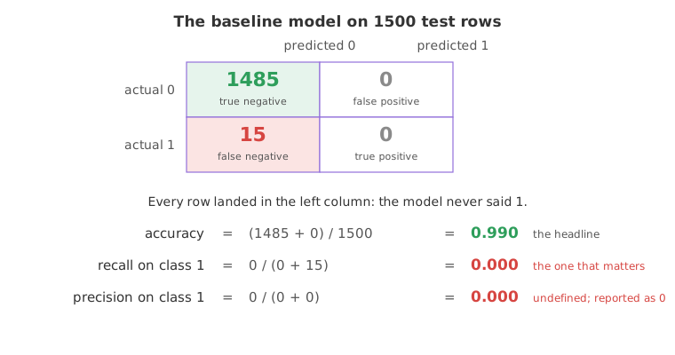
Comparing the model with a rule that always answers zero
DummyClassifier(strategy="most_frequent") learns one thing: which label is commonest. It then returns that label for every row. If a real model cannot beat it, the real model has learned nothing a user can act on.
from sklearn.dummy import DummyClassifier
from sklearn.metrics import accuracy_score, roc_auc_score

dummy = DummyClassifier(strategy="most_frequent").fit(X_train, y_train)

print("always answer 0:", accuracy_score(y_test, dummy.predict(X_test)))
print("the model:      ", accuracy_score(y_test, pred))
print()
scores = model.predict_proba(X_test)[:, 1]
print("highest score given to any test row:", round(scores.max(), 4))
print("model ROC AUC:", round(roc_auc_score(y_test, scores), 4))always answer 0: 0.99 the model: 0.99 highest score given to any test row: 0.4824 model ROC AUC: 0.9779
Reading the 99 per cent
- Accuracy matched a rule that ignores every feature. Both scored 0.99, because 99 per cent of the test rows are class 0 and both answered 0 for all of them.
- Recall on class 1 is zero. Fifteen minority rows were in the test set and none was found. For a fraud detector that is every fraud missed.
- Precision on class 1 is undefined. There were no positive predictions at all, so there is nothing to be right or wrong about. scikit-learn reports it as 0.
- The model is not blind. Its ROC AUC is about 0.98, which means it scores most minority rows above most majority rows. It ranks well and decides badly, because its highest score on any test row is still below the 0.5 cut-off that
predictuses. - That last point is the whole part. The signal is there. Three different ways of getting at it follow.
Accuracy against the metrics that survive imbalance
| Metric | What it answers | On a 99 to 1 target |
|---|---|---|
| Accuracy | What share of all rows did I label correctly? | Useless. 0.99 is the score for answering 0 every time. |
| Recall on the rare class | Of the rare rows that exist, how many did I find? | The headline number. 0.00 here. |
| Precision on the rare class | Of the rows I flagged, how many were right? | The cost side. Undefined here, because nothing was flagged. |
| F1 on the rare class | One number balancing the two above. | The usual single score to compare methods. |
| ROC AUC | Does the model score rare rows above common ones? | Judges the ranking, not the 0.5 cut-off. 0.98 here. |
| Confusion matrix | The four raw counts. | Always print it. A column of zeros is visible at once. |
Where imbalanced targets turn up
- Fraud and abuse. A few hundred fraudulent card payments among hundreds of thousands of honest ones.
- Manufacturing defects. A line that is working well produces very few failing parts, which is exactly why the failures are hard to learn.
- Churn, default and conversion. Most customers stay, most loans are repaid, most visitors do not buy, and the minority is the business question.
DummyClassifier score beside your own as the floor you have to clear.Related
- Previous: Cyclical encoding for hours and weekdays
- Next: Undersampling
- See also: class_weight
- Reference: Metrics and scoring in the scikit-learn user guide
- Set
class_sep=1.0inmake_classificationand refit. The classes pull apart and the same model suddenly finds all 15 minority rows, which shows that imbalance alone is not the problem; imbalance plus overlap is. - Change
weightsto[0.9, 0.1]and print the classification report again. Watch recall on class 1 rise as the minority stops being rare. - Drop
stratify=yfrom the split, run it five times with differentrandom_statevalues and printy_test.sum()each time.
Slow is fine. Stopping is the only problem.