
Mutual information
Mutual information measures how much knowing one column reduces the uncertainty about the target, counting any relationship at all rather than only a straight line.
Last updated: 12 Oct, 2026 · pandas 3.0 · scikit-learn 1.9
Dropping correlated features used Pearson correlation, which answers one question: as this column goes up, does the target go up or down in a straight line? A column can decide the target completely and still score zero on that question.
Mutual information is written I(X; Y) = H(Y) - H(Y | X). H(Y) is the uncertainty in the target on its own, and H(Y | X) is what is left once the column is known. The difference is how much the column told you. It is zero when the two are independent and grows with any kind of dependence, in either direction.
Syntax: two functions, one per target type, both of which need a seed.
from sklearn.feature_selection import mutual_info_classif, mutual_info_regression

mutual_info_classif(X, y, random_state=0)      # a target with classes
mutual_info_regression(X, y, random_state=0) # a continuous targetrandom_state= the scores move on every run. The ranking is stable; the digits are not. Always pass a seed before writing a number down.Catching what correlation cannot
A column drawn between minus three and three, with a target equal to its square plus noise, has a perfect relationship with that target. Pearson correlation reports almost nothing, because the target falls and then rises.
rng = np.random.default_rng(0)
x = rng.uniform(-3, 3, size=2000)
y = x ** 2 + rng.normal(scale=0.3, size=2000) # a U shape, not a lineimport numpy as np
import pandas as pd
from sklearn.feature_selection import mutual_info_regression
rng = np.random.default_rng(0)
x = rng.uniform(-3, 3, size=2000)
y = x ** 2 + rng.normal(scale=0.3, size=2000)
features = pd.DataFrame({"x": x, "abs_x": np.abs(x), "noise": rng.normal(size=2000)})
print("Pearson correlation with y:")
print(features.corrwith(pd.Series(y)).round(4).to_string())
print()
print("mutual information with y:")
print(pd.Series(mutual_info_regression(features, y, random_state=0),
index=features.columns).round(4).to_string())Pearson correlation with y: x -0.0128 abs_x 0.9630 noise 0.0081 mutual information with y: x 1.9883 abs_x 1.9554 noise 0.0249
xcorrelates at about minus 0.01 with the target, which reads as no relationship, and a correlation filter would drop it.xscores about 1.99 on mutual information, the highest of the three. The target is a function ofx, and mutual information sees that.abs_xcorrelates at 0.96, because taking the absolute value straightens the U into a line. The same information, differently written.- The noise column scores near zero on both. Mutual information is not uniformly larger for everything; it separates signal from nothing.
Ranking the house price columns
On the Ames data the target is a price, so mutual_info_regression is the function. The split comes first, so the scores are computed from training rows only, and fillna(0) handles the three numeric columns that still have missing values, because neither function accepts a NaN.
X_train, X_test, y_train, y_test = train_test_split(
    X, y, test_size=0.3, random_state=0)

scores = mutual_info_regression(X_train.fillna(0), y_train, random_state=0)
scores = pd.Series(scores, index=X_train.columns).sort_values(ascending=False)import pandas as pd
from sklearn.model_selection import train_test_split
from sklearn.feature_selection import mutual_info_regression
X_train, X_test, y_train, y_test = train_test_split(
X, y, test_size=0.3, random_state=0)
scores = mutual_info_regression(X_train.fillna(0), y_train, random_state=0)
scores = pd.Series(scores, index=X_train.columns).sort_values(ascending=False)
print(scores.head(10).round(4).to_string())
print()
print("columns scoring exactly zero:", int((scores == 0).sum()))
print(list(scores[scores == 0].index))OverallQual 0.5181 GrLivArea 0.4818 GarageCars 0.3853 TotalBsmtSF 0.3823 GarageArea 0.3646 YearBuilt 0.3512 1stFlrSF 0.3104 GarageYrBlt 0.2694 FullBath 0.2650 YearRemodAdd 0.2544 columns scoring exactly zero: 7 ['BsmtHalfBath', 'LowQualFinSF', '3SsnPorch', 'PoolArea', 'MiscVal', 'MoSold', 'YrSold']
OverallQualleads at about 0.52, followed byGrLivArea. Both are what a surveyor would name first.- Seven columns score exactly zero, including
YrSold,MoSoldandPoolArea. The estimator could not find any dependence at all. - A zero is a stronger statement than a low correlation. It says no relationship of any shape was detected, not only no straight line.
Comparing the two rankings
Drawing both scores on the same columns shows where they disagree, and the disagreements are where mutual information earns its place.
import numpy as np
import matplotlib.pyplot as plt

pearson = X_train.fillna(0).corrwith(y_train).abs()
order = scores.sort_values(ascending=False).head(12).index

fig, ax = plt.subplots(figsize=(8, 5))
position = np.arange(len(order))
ax.bar(position - 0.2, scores[order], 0.4, label="mutual information", color="#9370DB")
ax.bar(position + 0.2, pearson[order], 0.4, label="|Pearson correlation|", color="#b9bfd0")
ax.set_xticks(position, order, rotation=60, ha="right")
ax.set_ylabel("score against SalePrice")
ax.set_title("Mutual information and correlation do not agree")
ax.legend()
plt.show()
print("MSSubClass: mutual information", round(scores["MSSubClass"], 4),
" |Pearson|", round(pearson["MSSubClass"], 4))MSSubClass: mutual information 0.2478 |Pearson| 0.081
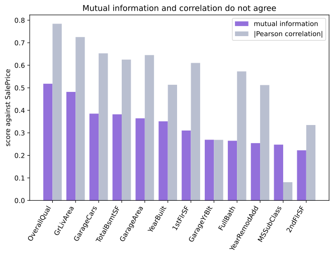
- The two bars usually move together. Both methods agree that
OverallQualandGrLivAreamatter most. MSSubClassbreaks the pattern. Mutual information puts it eleventh while correlation puts it twenty-seventh, with a correlation of about 0.08.- The reason is in what the column holds.
MSSubClassis a building class code: 20 means a one-storey house built in 1946 or later, 60 means a two-storey. The numbers are labels, and price does not rise with the code, so correlation sees nothing while mutual information sees a strong dependence. - A correlation filter would have dropped it. That is the failure mode this lesson exists to prevent.
Selecting on the scores
SelectKBest and SelectPercentile turn a score function into a transformer. The seed has to be bound into the score function, because these classes pass only X and y through.
from functools import partial
from sklearn.feature_selection import SelectPercentile, mutual_info_regression

seeded = partial(mutual_info_regression, random_state=0)
selector = SelectPercentile(seeded, percentile=20).fit(X_train.fillna(0), y_train)

print("kept", selector.get_support().sum(), "of", X_train.shape[1], "columns")
print(list(X_train.columns[selector.get_support()]))kept 7 of 36 columns ['OverallQual', 'YearBuilt', 'TotalBsmtSF', '1stFlrSF', 'GrLivArea', 'GarageCars', 'GarageArea']
Correlation against mutual information
| Pearson correlation | Mutual information | |
|---|---|---|
| Finds | Straight-line relationships | Any relationship, straight or not |
| Direction | Signed, so it says up or down | Unsigned, so it only says how much |
| Scale | Always between minus 1 and 1 | Zero upwards, with no fixed maximum |
| Reproducible | Exactly | Only with random_state= |
| Speed | One matrix multiplication | A nearest-neighbour search per column |
| Reads coded numbers | Badly; it treats a class code as a quantity | Correctly |
Where mutual information is the right filter
- Columns that are codes, not quantities. Postcodes, product ids, building classes and any other label that happens to be stored as an integer.
- Relationships with a turning point. Age against income, temperature against energy use, dose against effect.
- A first pass on a wide frame. It fits no model, so it ranks a thousand columns quickly, and what it keeps is then passed to a slower method.
Related
- Previous: Dropping correlated features
- Next: Chi square for categorical features
- See also: Model based selection with Lasso
- Reference: mutual_info_regression in the scikit-learn API reference
- Run
mutual_info_regressiontwice withoutrandom_stateand subtract the two arrays; the largest difference is the size of the noise you would have written into a report. - Change
n_neighborsonmutual_info_regressionfrom its default of 3 to 10 and see how far the top of the ranking moves. - Print
df["MSSubClass"].value_counts(), then drawdf.boxplot(column="SalePrice", by="MSSubClass")to see the relationship correlation missed. The price does not climb with the code, which is why Pearson scored it at 0.08.
Every expert started right here.