
Mean and median imputation
Mean or median imputation fills every missing value in a numeric column with one number worked out from the values that are present, which completes the column and shrinks its spread.
Last updated: 12 Oct, 2026 · pandas 3.0
Why values go missing argued that the Titanic ages look close to missing completely at random. That is the case this technique is for, and the cost of using it can be measured to four decimal places.
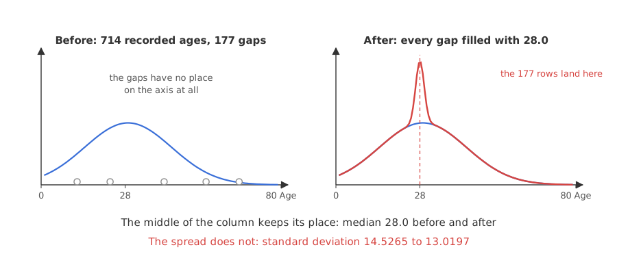
Syntax: Series.median() and Series.mean() compute the fill value from the non-missing rows, and Series.fillna(value) returns a new Series with the gaps filled. Assign the result back; an in-place fill through a column reference does nothing under copy-on-write, as Copy-on-write and chained assignment shows.
median = df['Age'].median()          # computed from the 714 recorded ages
df['Age_median'] = df['Age'].fillna(median)    # a new column, nothing lost
df['Age'] = df['Age'].fillna(median)           # or fill the column in place
df['Age'].fillna(median, inplace=True)         # does nothing: never write this
Loading the Titanic data
The Titanic table is 891 passengers. Age is missing for 177 of them, Cabin for 687 and Embarked for 2, which makes it the right table to learn these techniques on. It loads from its GitHub URL, so there is nothing to download. Run this block first, then the example under it.
import pandas as pd
import matplotlib
matplotlib.use('svg')
import matplotlib.pyplot as plt

url = ("https://raw.githubusercontent.com/krishnaik06/"
       "Feature-Engineering-Live-sessions/master/titanic.csv")
df = pd.read_csv(url, usecols=['Survived', 'Age', 'Fare'])
Filling 177 ages and measuring the damage
Filling into a new column rather than over the original keeps both versions side by side, which is what makes the comparison possible. The standard deviation and the correlation with the target are the two numbers worth reading afterwards.
median = df['Age'].median()
mean = df['Age'].mean()
print("median:", median, "  mean:", round(mean, 6))

df['Age_median'] = df['Age'].fillna(median)
df['Age_mean'] = df['Age'].fillna(mean)
print("nulls left:", int(df['Age_median'].isnull().sum()))
print("std before:      ", df['Age'].std())
print("std after median:", df['Age_median'].std())
print("corr with Survived before:", round(df['Age'].corr(df['Survived']), 6))
print("corr with Survived after: ", round(df['Age_median'].corr(df['Survived']), 6))median: 28.0 mean: 29.699118 nulls left: 0 std before: 14.526497332334042 std after median: 13.019696550973201 corr with Survived before: -0.077221 corr with Survived after: -0.06491
Reading the four numbers
- The median is 28.0 and the mean is 29.699118. They are close, so Age is close to symmetric and either would do. On a skewed column they would be far apart.
- The standard deviation falls from 14.526497 to 13.019697. 177 values that used to be spread out are now all exactly 28.0, so the spread shrinks by about 10 percent.
- The correlation with Survived weakens from -0.077221 to -0.064910. The relationship the column had with the target is diluted by 177 rows that now carry no information.
- Nothing warns you. The column is complete, the code ran, and the two numbers above are the only evidence that anything was lost.
Seeing the spike the fill creates
A KDE curve of the column before and after the fill shows where the damage lands. The two curves agree everywhere except around the fill value, where the new one has a spike that the data never had.
df['Age_median'] = df['Age'].fillna(df['Age'].median())
print("passengers aged exactly 28.0 before:", int((df['Age'] == 28.0).sum()))
print("passengers aged exactly 28.0 after: ",
      int((df['Age_median'] == 28.0).sum()))

fig, ax = plt.subplots(figsize=(7, 4))
df['Age'].plot(kind='kde', ax=ax, label='Age, the 714 recorded')
df['Age_median'].plot(kind='kde', ax=ax, color='red',
                      label='Age after filling 177 with 28.0')
ax.set_xlabel('Age')
ax.legend()
ax.set_title('What one fill value does to the shape')
fig.savefig('chart.svg')passengers aged exactly 28.0 before: 25 passengers aged exactly 28.0 after: 202
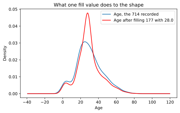
25 passengers were recorded as exactly 28.0; after the fill 202 are. The red curve's peak is those extra 177 rows, and anything that reads the shape of this column now sees a spike that no passenger created.
Mean vs median vs mode
| Mean | Median | Mode | |
|---|---|---|---|
| Fill value | the average of the present values | the middle value | the most frequent value |
| Column type | numeric | numeric | categorical or discrete |
| Outliers move it | yes, a great deal | hardly | no |
| Skewed column | pulled into the tail | stays with the bulk | not applicable |
| Creates a value that never existed | often, 29.699118 is nobody's age | no, the median is a real value here | no |
| Taught in | this lesson | this lesson | Frequent category imputation |
The median is the default choice for a numeric column with any skew or any outliers, which is most numeric columns. Fare is the clear case: its mean sits above its third quartile, so filling a gap in it with the mean would place that passenger above three quarters of the fares the passengers paid.
Where mean and median imputation fit
- A column with a few percent missing, no pattern to the gaps. The fastest complete fix, and the cost is small when the share is small.
- A baseline before anything cleverer. Fit a model on median filled columns first; every later technique has to beat it.
- Inside a pipeline.
SimpleImputer(strategy='median')is the same calculation with the fill value learned on the training set only, which is what SimpleImputer in scikit-learn is for.
Related
- Previous: Why values go missing
- Next: Random sample imputation
- See also: SimpleImputer in scikit-learn
- Reference: Series.fillna in the pandas docs
- Fill with the mean instead of the median and compare the two standard deviations.
- Run the same comparison on
Fareafter setting 100 of its values to NaN withdf.loc[df.sample(100, random_state=0).index, 'Fare'] = None. - Write
df['Age'].fillna(28, inplace=True)and then printdf['Age'].isnull().sum()to see that nothing happened.
This is what real progress feels like.