
Project: the feature selection
The selection step fits a Lasso on the 82 prepared training columns and keeps the 21 whose coefficients did not shrink to zero.
Last updated: 12 Oct, 2026 · pandas 3.0 · scikit-learn 1.9
Project: building the features produced 82 columns for 1,314 houses. Most of them say almost nothing about the price, and a model with 82 coefficients fitted on 1,314 rows is a model with a lot of room to memorise. Model based selection with Lasso introduced the technique; this is it applied to the project, with the fit on the training rows.
The feature pass this lesson starts from
Nothing here is new. It is the pass from the previous lesson, unchanged, and it ends with train_ready, test_ready and the two log prices.
import numpy as np
import pandas as pd
from sklearn.model_selection import train_test_split
from sklearn.preprocessing import MinMaxScaler

AMES = ("https://raw.githubusercontent.com/krishnaik06/"
        "Advanced-House-Price-Prediction-/master/train.csv")
houses = pd.read_csv(AMES)
y = np.log(houses['SalePrice'])
X = houses.drop(columns=['Id', 'SalePrice'])
X_train, X_test, y_train, y_test = train_test_split(
    X, y, test_size=0.1, random_state=0)

NANCOLS = ['LotFrontage', 'MasVnrArea', 'GarageYrBlt']
YEARS = ['YearBuilt', 'YearRemodAdd', 'GarageYrBlt']
LOGS = ['LotFrontage', 'LotArea', '1stFlrSF', 'GrLivArea']

def flags(frame):
    frame = frame.copy()
    for c in NANCOLS:
        frame[c + 'nan'] = frame[c].isnull().astype(int)
    return frame

def ages_and_logs(frame):
    frame = frame.copy()
    for c in YEARS:
        frame[c] = frame['YrSold'] - frame[c]
    for c in LOGS:
        frame[c] = np.log(frame[c])
    return frame

train, test = flags(X_train), flags(X_test)
numbers = [c for c in train.columns if pd.api.types.is_numeric_dtype(train[c])]
words = [c for c in train.columns if pd.api.types.is_string_dtype(train[c])]

medians = train[numbers].median()
train[numbers] = train[numbers].fillna(medians)
test[numbers] = test[numbers].fillna(medians)

train, test = ages_and_logs(train), ages_and_logs(test)
train[words] = train[words].fillna('Missing')
test[words] = test[words].fillna('Missing')

codes = {}
for c in words:
    share = train[c].value_counts(normalize=True)
    keep = share[share > 0.01].index
    train[c] = np.where(train[c].isin(keep), train[c], 'Rare_var')
    test[c] = np.where(test[c].isin(keep), test[c], 'Rare_var')
    order = y_train.groupby(train[c]).mean().sort_values().index
    codes[c] = {label: i for i, label in enumerate(order)}
    train[c] = train[c].map(codes[c]).astype(float)
    test[c] = pd.Series(test[c], index=test.index).map(codes[c]).fillna(-1).astype(float)

features = numbers + words
scaler = MinMaxScaler().set_output(transform='pandas').fit(train[features])
train_ready = scaler.transform(train[features])
test_ready = scaler.transform(test[features])
Letting a Lasso decide
A Lasso adds a penalty on the size of the coefficients, and that penalty drives the useless ones to exactly zero rather than merely small. SelectFromModel wraps it and keeps the columns that survive. alpha=0.005 sets how hard the penalty pushes: larger keeps fewer columns. random_state=0 makes the fit repeatable.
chooser = SelectFromModel(Lasso(alpha=0.005, random_state=0))
chooser.fit(train_ready, y_train)          # the training rows, once more
kept = train_ready.columns[chooser.get_support()]
Cutting 82 columns down to 21
from sklearn.feature_selection import SelectFromModel
from sklearn.linear_model import Lasso
from sklearn.metrics import r2_score

chooser = SelectFromModel(Lasso(alpha=0.005, random_state=0))
chooser.fit(train_ready, y_train)
kept = train_ready.columns[chooser.get_support()]
print("features offered:", train_ready.shape[1])
print("features kept:", len(kept))
print("coefficients shrunk to zero:", int((chooser.estimator_.coef_ == 0).sum()))
print(sorted(kept.tolist()))

model_all = Lasso(alpha=0.005, random_state=0).fit(train_ready, y_train)
model_few = Lasso(alpha=0.005, random_state=0).fit(train_ready[kept], y_train)
print("test R2 with all 82:", round(r2_score(y_test, model_all.predict(test_ready)), 4))
print("test R2 with the 21:", round(r2_score(y_test, model_few.predict(test_ready[kept])), 4))features offered: 82 features kept: 21 coefficients shrunk to zero: 61 ['1stFlrSF', 'BsmtExposure', 'BsmtFullBath', 'BsmtQual', 'CentralAir', 'FireplaceQu', 'Fireplaces', 'GarageCars', 'GarageFinish', 'GarageType', 'GrLivArea', 'HeatingQC', 'KitchenQual', 'MSSubClass', 'MSZoning', 'Neighborhood', 'OverallCond', 'OverallQual', 'PavedDrive', 'RoofStyle', 'YearRemodAdd'] test R2 with all 82: 0.8592 test R2 with the 21: 0.8592
- 61 of the 82 coefficients are exactly zero. Not small, zero. That is what the Lasso penalty does and why it can be used to choose columns rather than only to fit them.
- The 21 survivors read like a house description. The living area, the first floor, the overall quality and condition, the neighbourhood, the zoning, the kitchen and basement grades, the garage and the fireplace. Nothing in that list is a surprise, which is the point: the method agrees with what a person would guess, having been told nothing.
- The score is the same either way, 0.8592. Dropping 61 columns cost nothing on the held back houses, because those columns were contributing nothing. The gain is a smaller model, fewer values to collect and less to go wrong when it is served.
Plotting the 82 coefficients
import matplotlib
matplotlib.use('svg')
import matplotlib.pyplot as plt
from sklearn.feature_selection import SelectFromModel
from sklearn.linear_model import Lasso

chooser = SelectFromModel(Lasso(alpha=0.005, random_state=0)).fit(train_ready, y_train)
coefs = pd.Series(chooser.estimator_.coef_, index=train_ready.columns)
order = coefs.abs().sort_values(ascending=False)
print("largest three:", order.head(3).round(4).to_dict())
print("exactly zero:", int((coefs == 0).sum()))

vals = coefs[order.index]
fig, ax = plt.subplots(figsize=(8, 4.5))
ax.bar(range(len(vals)), vals.values,
       color=['#2e9e5b' if v != 0 else '#cccccc' for v in vals.values])
ax.axhline(0, color='#333', linewidth=1)
ax.annotate('61 columns, coefficient exactly 0', xy=(50, 0.03), color='#777')
ax.set_xlabel('the 82 columns, ordered by the size of the coefficient')
ax.set_ylabel('Lasso coefficient')
ax.set_title('21 coefficients survive, 61 are exactly zero')
fig.tight_layout()
fig.savefig('chart.svg')largest three: {'GrLivArea': 0.7302, 'OverallQual': 0.4368, 'Neighborhood': 0.3274}
exactly zero: 61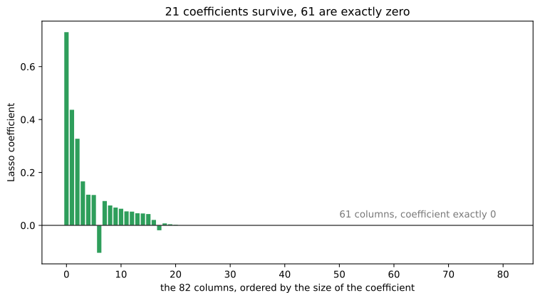
- Three columns carry most of the price. The living area at 0.7302, the overall quality at 0.4368 and the neighbourhood at 0.3274, all on the scaled 0 to 1 range so the sizes are comparable.
- One bar points down.
YearRemodAddbecame an age in the feature pass, so a larger value means a remodel further in the past, and its coefficient is negative at -0.1036. A sign is a direction, not a weakness. - The curve falls away fast. The twenty first surviving column,
OverallCond, has a coefficient of 0.0020 against the first column's 0.7302, which is why 21 is a soft number: a slightly larger alpha would stop sooner. - The grey block is flat, not nearly flat. A ridge penalty would leave 82 small bars; the Lasso leaves 21 and a floor.
All 82 columns against the 21
| Keep all 82 | Keep the 21 | |
|---|---|---|
| Test R squared | 0.8592 | 0.8592 |
| Coefficients to store | 82, 61 of them zero | 21 |
| Values to collect to score one house | every column in the file | 21 of them |
| What a reader learns from the model | little, the list is the whole table | which parts of a house set its price |
| Risk when a column changes upstream | any of 82 can break it | 21 can |
Where a selection step belongs
- When columns cost money or time to collect. A model that needs 21 values instead of 82 is cheaper to feed, every day it runs.
- When the model has to be explained. Twenty one named columns with signed coefficients is a conversation; 82 is a dump.
- Inside cross-validation, never before it. The selection is fitted here on the training rows only, and the next lesson moves it inside a pipeline so that stays true in every fold.
Related
- Previous: Project: building the features
- Next: Project: the whole thing as one pipeline
- See also: Why features are dropped
- Reference: Feature selection in the scikit-learn documentation
- Set
alpha=0.05and count the survivors. A ten times larger penalty leaves three columns and the test R squared falls to 0.3555. - Set
alpha=0.0005and count again. Fifty four columns survive and the test R squared reaches 0.8879, so the question is no longer which columns to keep but how small a model you want. - Print
coefs[kept].sort_values().YearRemodAddsits at the bottom with -0.1036: an age runs the other way from the price.
Every expert started right here.