
Finding outliers with the z score
The z score of a value is how many standard deviations it sits from the mean of its column, and the usual rule calls a value an outlier when its z score is past 3 in either direction.
Last updated: 12 Oct, 2026 · pandas 3.0 · scikit-learn 1.9
What an outlier is picked the three far readings out by eye with a cut-off of 50. This lesson replaces the eye with a rule that reads the column and decides for itself.
Syntax: the z score is a subtraction and a division, so it needs no library beyond the one computing the mean and the standard deviation.
Scoring the 34 readings
The mean and the standard deviation
values.mean() and values.std() on a NumPy array divide by n. Series.std() in pandas divides by n minus 1 and gives 26.7689 for the same column. Both answers are correct; they are different conventions, and the one you pick shifts every z score slightly.
mean, std = values.mean(), values.std() # NumPy divides by nThe score of every value, and the threshold
Subtracting the mean and dividing by the standard deviation turns the column into scores centred on zero. abs catches both tails at once, so a value far below the mean is flagged on the same rule as a value far above.
z = (values - mean) / std
outliers = [int(v) for v, score in zip(values, z) if abs(score) > 3]
Running the 3 rule on the readings
import numpy as np

readings = [11, 10, 12, 14, 12, 15, 14, 13, 15, 102, 12, 14, 17, 19, 107,
            10, 13, 12, 14, 12, 108, 12, 11, 14, 13, 15, 10, 15, 12, 10, 14, 13, 15, 10]
values = np.array(readings)
mean, std = values.mean(), values.std()   # NumPy divides by n

z = (values - mean) / std
outliers = [int(v) for v, score in zip(values, z) if abs(score) > 3]

print("mean:", round(mean, 4), " std:", round(std, 4))
print("largest |z|:", round(np.abs(z).max(), 4))
print("outliers:", outliers)mean: 21.1765 std: 26.3723 largest |z|: 3.2922 outliers: [102, 107, 108]
Reading the three scores
- The mean is 21.1765 and the standard deviation 26.3723. Both numbers were computed from the column that contains the three far values, so the rule is measuring the readings against a centre and a spread those same readings pushed out of place.
- The largest score is 3.2922. That belongs to 108, the largest reading. It clears 3, so the rule fires.
- Three values are flagged: 102, 107 and 108. The same three the dot plot showed.
- The 3 is a choice. For a normal column, about 99.7% of values fall inside 3 standard deviations, so a threshold of 3 flags roughly 3 values in 1000. Lower it to 2 and the rule flags about 5 in 100.
The same test with scipy.stats.zscore
SciPy writes the same arithmetic in one call. Its ddof argument is the same n or n minus 1 choice, and it defaults to 0, which is the NumPy convention used above.
import numpy as np
from scipy import stats

readings = [11, 10, 12, 14, 12, 15, 14, 13, 15, 102, 12, 14, 17, 19, 107,
            10, 13, 12, 14, 12, 108, 12, 11, 14, 13, 15, 10, 15, 12, 10, 14, 13, 15, 10]
values = np.array(readings)

z = stats.zscore(values)                 # ddof=0, the same as NumPy's std
print("same scores:", np.allclose(z, (values - values.mean()) / values.std()))
print("threshold 3:", [int(v) for v in values[np.abs(z) > 3]])
print("threshold 2:", [int(v) for v in values[np.abs(z) > 2]])same scores: True threshold 3: [102, 107, 108] threshold 2: [102, 107, 108]
Lowering the threshold to 2 returns the same three values here. The gap between 19 and 102 is wide enough that no reasonable threshold lands inside it.
Drawing the boundaries on a real column
Working with the two boundaries is often easier than working with the scores: a z score past 3 is the same as a value outside mean plus or minus 3 standard deviations. On the Titanic Age column those boundaries are a number you can read off a histogram.
import matplotlib
matplotlib.use("svg")
import matplotlib.pyplot as plt
import pandas as pd

URL = ("https://raw.githubusercontent.com/krishnaik06/Feature-Engineering-Live-sessions/"
       "master/titanic.csv")
age = pd.read_csv(URL)["Age"].dropna()

lower = age.mean() - 3 * age.std()
upper = age.mean() + 3 * age.std()
print("mean:", round(age.mean(), 6), " std:", round(age.std(), 6))
print("lower:", lower)
print("upper:", upper)
print("ages outside:", sorted(age[(age < lower) | (age > upper)].tolist()))

fig, ax = plt.subplots(figsize=(7, 3.1))
ax.hist(age, bins=40, color="#9370DB", edgecolor="white")
ax.axvline(lower, color="#d64541", linestyle="--", label="mean - 3 x std")
ax.axvline(upper, color="#d64541", linestyle="--", label="mean + 3 x std")
ax.set_xlabel("Age")
ax.set_ylabel("passengers")
ax.legend()
fig.savefig("chart.svg")mean: 29.699118 std: 14.526497 lower: -13.880374349943303 upper: 73.27860964406094 ages outside: [74.0, 80.0]
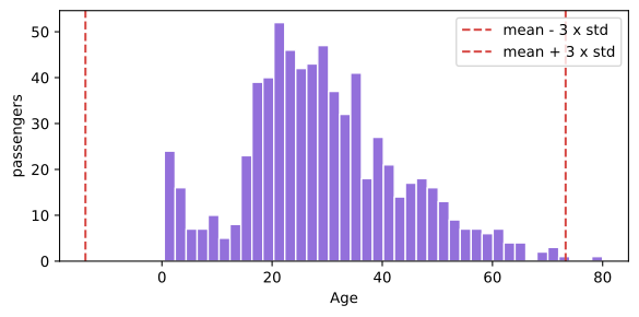
The lower boundary is minus 13.88, an age that cannot exist, so the rule flags nothing on the left. On the right it flags two passengers, aged 74 and 80. Both are plausible ages and neither is an error, which is the point made earlier: the rule finds candidates, not verdicts.
The assumption the rule makes
Mean plus or minus 3 standard deviations only means 99.7% of the column when the column is close to normal. On a column with a long right tail, the mean and the standard deviation are both pulled towards the tail, the boundary runs away with them, and the rule stops flagging anything.
import pandas as pd

URL = ("https://raw.githubusercontent.com/krishnaik06/Feature-Engineering-Live-sessions/"
       "master/titanic.csv")
df = pd.read_csv(URL)

for col in ["Age", "Fare"]:
    s = df[col].dropna()
    upper = s.mean() + 3 * s.std()
    print(f"{col:5s} skew {s.skew():6.3f}   mean+3*std {upper:8.3f}"
f" max {s.max():8.3f} flagged {(s > upper).sum():4d}")Age skew 0.389 mean+3*std 73.279 max 80.000 flagged 2 Fare skew 4.787 mean+3*std 181.284 max 512.329 flagged 20
Why Fare defeats the rule
- Age has a skew of 0.389. Close enough to symmetric for the rule to behave: the boundary lands at 73.3, inside the range of the column, and flags 2 of 714 rows.
- Fare has a skew of 4.787. A long right tail. The standard deviation is 49.69, larger than the mean of 32.20, so the boundary lands at 181.28.
- 181.28 is above the 99.9th percentile of the column. The rule flags 20 fares out of 891, and the fence in the next lesson flags 116.
- The tail moved the rule, not the other way round. The same values the rule should catch are the ones that pushed the boundary past themselves.
Z score vs the IQR fence
| Z score | IQR fence | |
|---|---|---|
| Built from | the mean and the standard deviation | the 25th and 75th percentiles |
| Moved by the values it is testing | yes, both inputs are | no, percentiles are positions |
| Use it when | the column is roughly symmetric | the column is skewed, or you do not know |
| Usual threshold | |z| > 3, sometimes 2 | outside Q1 - 1.5 x IQR to Q3 + 1.5 x IQR |
| On Titanic Fare | 20 rows flagged, boundary at 181.28 | 116 rows flagged, fence at 65.63 |
Where the z score is the right rule
- Sensor and measurement data. Readings of one physical quantity usually scatter symmetrically around a true value, which is the shape the rule assumes.
- Residuals from a fitted model. The errors of a well-fitted regression are meant to be symmetric around zero, so a residual with a large z score points at a row the model cannot explain.
- Any column after a successful Gaussian transformation. Once a skewed column has been transformed towards normal, the rule applies to the transformed values.
Related
- Previous: What an outlier is
- Next: The IQR fence
- See also: Log, reciprocal and square root transformations
- Reference: scipy.stats.zscore
- Change the threshold from 3 to 1.5 in the readings example and print how many values are flagged.
- Pass
ddof=1tostats.zscoreand compare the largest score with the 3.2922 printed above. - Run the boundary example on
Farein place ofAgeand look at where the two dashed lines land on the histogram.
Slow is fine. Stopping is the only problem.