
Data leakage
Data leakage is a number or a decision in your preparation that came from rows you are going to be scored on, so the score you measure is better than the score you will get.
Last updated: 12 Oct, 2026 · pandas 3.0 · scikit-learn 1.9
Every technique in this course so far was fitted on a whole table: a median, a mode, a minimum and maximum, a label order, a list of columns worth keeping. That is fine while you are looking at data. It stops being fine the moment you measure how good a model is, because the measurement is supposed to stand in for rows you have never seen. This lesson causes the problem twice and puts a number on it.
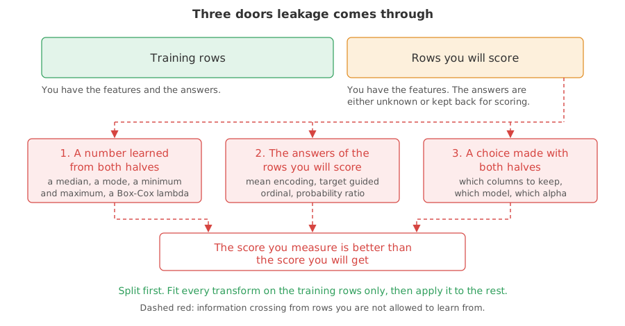
Naming the three doors
- A number learned from every row. A median used to fill gaps, the minimum and maximum a scaler divides by, the mode of a text column, the lambda Box-Cox picked. Each one is a summary of the rows it saw, and the rows you will score were among them.
- The answers of the rows you will score. Target guided ordinal encoding, mean encoding and probability ratio encoding all read the target. Computed over the whole table, they write a piece of each row's own answer into that row's features.
- A choice made with every row. Which columns to keep, which model, which alpha. A choice is information too, and a choice made while looking at the scored rows is as leaky as a number.
The cure is the same in all three cases and it is one rule: split first, learn everything from the training rows, then apply what you learned to the rest.
Building a table with no signal in it
The cleanest way to see a leak is to make data where any score above chance is wrong. Three hundred rows, a thousand columns of random numbers and a coin-flip target. No column has anything to do with the answer, so an honest model cannot beat 0.5.
rng = np.random.default_rng(0)                 # seeded, so two runs agree
X = pd.DataFrame(rng.normal(size=(300, 1000)),
                 columns=[f"f{i}" for i in range(1000)])
y = pd.Series(rng.integers(0, 2, size=300))    # 0 or 1, unrelated to X
Scoring the columns before and after the split
SelectKBest(f_classif, k=20) keeps the twenty columns whose means differ most between the two classes. The leaky order runs it on all three hundred rows and then splits. The honest order splits first and runs it on the training half only. Everything else is identical, down to the random_state.
def two_scores(seed):
    rng = np.random.default_rng(seed)
    X = pd.DataFrame(rng.normal(size=(300, 1000)),
                     columns=[f"f{i}" for i in range(1000)])
    y = pd.Series(rng.integers(0, 2, size=300))
    keep = X.columns[SelectKBest(f_classif, k=20).fit(X, y).get_support()]
    a, b, ya, yb = train_test_split(X[keep], y, test_size=0.3, random_state=0)
    leaky = accuracy_score(yb, LogisticRegression().fit(a, ya).predict(b))
    a, b, ya, yb = train_test_split(X, y, test_size=0.3, random_state=0)
    keep2 = a.columns[SelectKBest(f_classif, k=20).fit(a, ya).get_support()]
    honest = accuracy_score(yb, LogisticRegression().fit(a[keep2], ya).predict(b[keep2]))
    return leaky, honest
Running the two orders on noise
import numpy as np
import pandas as pd
from sklearn.feature_selection import SelectKBest, f_classif
from sklearn.linear_model import LogisticRegression
from sklearn.metrics import accuracy_score
from sklearn.model_selection import train_test_split

def two_scores(seed):
    rng = np.random.default_rng(seed)
    X = pd.DataFrame(rng.normal(size=(300, 1000)),
                     columns=[f"f{i}" for i in range(1000)])
    y = pd.Series(rng.integers(0, 2, size=300))
    keep = X.columns[SelectKBest(f_classif, k=20).fit(X, y).get_support()]
    a, b, ya, yb = train_test_split(X[keep], y, test_size=0.3, random_state=0)
    leaky = accuracy_score(yb, LogisticRegression().fit(a, ya).predict(b))
    a, b, ya, yb = train_test_split(X, y, test_size=0.3, random_state=0)
    keep2 = a.columns[SelectKBest(f_classif, k=20).fit(a, ya).get_support()]
    honest = accuracy_score(yb, LogisticRegression().fit(a[keep2], ya).predict(b[keep2]))
    return leaky, honest

leaky, honest = two_scores(0)
print("leaky  accuracy:", round(leaky, 4))
print("honest accuracy:", round(honest, 4))leaky accuracy: 0.7111 honest accuracy: 0.3889
- 0.7111 from pure noise. The leaky order found twenty columns that happened to line up with the answer across all three hundred rows. The test rows were part of that search, so the columns were chosen to suit them.
- 0.3889 when the search is honest. The honest order looked for columns using the training rows only. The twenty it found mean nothing on the test rows, and the score lands near chance, sometimes a little above it and sometimes below.
- The gap is the leak. Nothing in the data changed. Only the order of the split and the search.
Checking that the gap is not one lucky seed
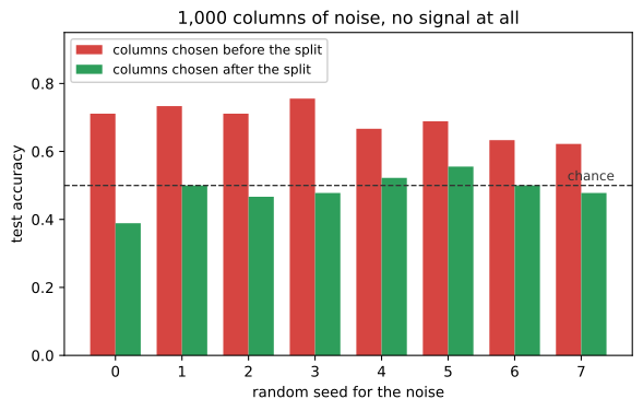
One pair of numbers proves nothing. Building the same table from eight different random seeds and plotting both scores shows the leaky bar sitting well above the dashed chance line every time, while the honest bar wanders around it.
import matplotlib
matplotlib.use('svg')
import matplotlib.pyplot as plt

seeds = range(8)
pairs = [two_scores(s) for s in seeds]
leaky = [p[0] for p in pairs]
honest = [p[1] for p in pairs]
print("leaky :", [round(v, 3) for v in leaky])
print("honest:", [round(v, 3) for v in honest])

fig, ax = plt.subplots(figsize=(7, 4))
w = 0.38
ax.bar([s - w / 2 for s in seeds], leaky, w, color='#d64541',
       label='columns chosen before the split')
ax.bar([s + w / 2 for s in seeds], honest, w, color='#2e9e5b',
       label='columns chosen after the split')
ax.axhline(0.5, color='#333', linestyle='--', linewidth=1)
ax.text(7.5, 0.515, 'chance', color='#333', ha='right', fontsize=9)
ax.set_ylim(0, 0.95)
ax.set_xticks(list(seeds))
ax.set_xlabel('random seed for the noise')
ax.set_ylabel('test accuracy')
ax.set_title('1,000 columns of noise, no signal at all')
ax.legend(loc='upper left', fontsize=9, framealpha=1)
fig.savefig('chart.svg')leaky : [0.711, 0.733, 0.711, 0.756, 0.667, 0.689, 0.633, 0.622] honest: [0.389, 0.5, 0.467, 0.478, 0.522, 0.556, 0.5, 0.478]
A target encoder that memorised the answer
Noise makes the point loudly. The second demonstration is the leak you will meet for real, on the Titanic table, with a technique this course teaches: a code per label taken from the mean of the target. The Ticket column has 681 different tickets among 891 passengers, and 547 of them belong to a single passenger. A mean over one row is that row's own answer.
# the leaky order: one mean per ticket, taken over every row
mean_all = y.groupby(df['Ticket']).mean()
X = df[['Pclass', 'Fare']].assign(Ticket_enc=df['Ticket'].map(mean_all))# the honest order: split first, means from the training half only
mean_train = ya.groupby(a['Ticket']).mean()
fallback = ya.mean() # for a ticket the training half never sawimport pandas as pd
from sklearn.metrics import accuracy_score
from sklearn.model_selection import train_test_split
from sklearn.tree import DecisionTreeClassifier
URL = ("https://raw.githubusercontent.com/krishnaik06/"
"Feature-Engineering-Live-sessions/master/titanic.csv")
df = pd.read_csv(URL)
y = df['Survived']
cols = ['Pclass', 'Fare', 'Ticket']
counts = df['Ticket'].value_counts()
print("different tickets:", len(counts),
"held by a single passenger:", int((counts == 1).sum()))
# the leaky order: one mean per ticket, taken over every row
mean_all = y.groupby(df['Ticket']).mean()
X = df[['Pclass', 'Fare']].assign(Ticket_enc=df['Ticket'].map(mean_all))
a, b, ya, yb = train_test_split(X, y, test_size=0.3, random_state=0)
tree = DecisionTreeClassifier(max_depth=4, random_state=0).fit(a, ya)
print("leaky accuracy:", round(accuracy_score(yb, tree.predict(b)), 4))
# the honest order: split first, means from the training half only
a, b, ya, yb = train_test_split(df[cols], y, test_size=0.3, random_state=0)
mean_train = ya.groupby(a['Ticket']).mean()
fallback = ya.mean() # for a ticket the training half never saw
a2 = a.assign(Ticket_enc=a['Ticket'].map(mean_train)).drop(columns='Ticket')
b2 = b.assign(Ticket_enc=b['Ticket'].map(mean_train).fillna(fallback)).drop(columns='Ticket')
tree = DecisionTreeClassifier(max_depth=4, random_state=0).fit(a2, ya)
print("honest accuracy:", round(accuracy_score(yb, tree.predict(b2)), 4))
alone = b['Ticket'].map(counts) == 1
print("test rows whose ticket is theirs alone:", int(alone.sum()), "of", len(b))
print("their leaky code equals their own label:",
bool((X.loc[b.index[alone], 'Ticket_enc'].to_numpy() == yb[alone].to_numpy()).all()))
print("test tickets never seen in training:", int(b['Ticket'].map(mean_train).isnull().sum()))different tickets: 681 held by a single passenger: 547 leaky accuracy: 0.9179 honest accuracy: 0.7164 test rows whose ticket is theirs alone: 166 of 268 their leaky code equals their own label: True test tickets never seen in training: 177
- 0.9179 looks like a good model. It is a lookup table. For 166 of the 268 test passengers the ticket belongs to nobody else, so their code is their own survival value, and the last line confirms that every one of those codes equals the label the tree was asked to predict.
- 0.7164 is the model. Fitted the same way on the same rows, with the means taken from the training half, the tree gets the score it will get on real passengers.
- 177 test tickets were never in the training half. An honest encoder has to answer for them, which is why the code above fills them with the training mean. The leaky version never faces the question, which is part of why it flatters itself.
The leaky order against the honest order
| Fit on everything, then split | Split, then fit on train | |
|---|---|---|
| Noise table, 1,000 useless columns | 0.7111 | 0.3889 |
| Titanic, ticket mean encoding | 0.9179 | 0.7164 |
| What the number means | how well the pipeline fits rows it has already seen | how well it does on rows it has not |
| What you learn when the score is bad | nothing, the score was never real | which step to change |
| What happens in production | the score drops and nobody knows why | the score holds |
Where leakage hides in real work
- An identifier used as a feature. A ticket, a customer id, a booking reference. Encoded against the target it is a key into the answer sheet, as the Titanic run shows.
- A column recorded after the thing you predict. A refund amount when predicting a cancellation, a discharge code when predicting a diagnosis. No split protects you from this one, only reading what each column means and when it is written.
- A pass of cleaning before anything else. Filling, scaling and dropping correlated columns on the whole file at the top of a notebook, then splitting further down, is the most common version, and the most invisible.
Related
- Previous: Model based selection with Lasso
- Next: Split first, then fit
- See also: Mean encoding and Target guided ordinal encoding
- Reference: Common pitfalls and recommended practices in the scikit-learn documentation
- Change
size=(300, 1000)tosize=(3000, 1000)and the twosize=300arguments to 3000. The leaky score falls to 0.58, because a column that lines up with the answer across 3,000 coin flips is far rarer than one that does it across 300. - Drop the number of columns from 1000 to 50 in the noise table. The leaky score falls to 0.5889, because with fifty candidates there are fewer accidents to pick from.
- In the Titanic example, swap
TicketforEmbarked, which has three labels. The two accuracies land on the same number: a mean over hundreds of rows gives away nothing about any single one of them.
Slow is fine. Stopping is the only problem.