
Counting categories with value_counts
value_counts() is a Series method that returns how many rows carry each distinct value, as a new Series whose index is the values and whose numbers are the counts, sorted from the most common down.
Last updated: 12 Oct, 2026 · pandas 3.0 · seaborn 0.13 · matplotlib 3.11
One chart, one question, one observation drew its chart from one call to value_counts(). It is the first thing to run on any text or coded column, and the answer it gives has more in it than the counts.
Syntax: Series.value_counts() counts the distinct values. normalize=True turns counts into shares, dropna=False counts the missing values as a group of their own, and sort=False leaves the values in the order pandas found them.
counts = df['Country'].value_counts()   # a Series: value -> count
counts.index                            # the distinct values
counts.values                           # the counts, as a numpy array
df['Country'].value_counts(normalize=True)   # shares that add up to 1
df['Country'].value_counts(dropna=False)     # NaN counted as a group
Loading the Zomato data
Every example here starts from the merged Zomato frame. The zip recipe is the one Reading a CSV that is not UTF-8 built, and the join on the country code is the one Merging a lookup table built. Run this block first, then the example under it.
import io, zipfile, urllib.request
import pandas as pd
import matplotlib
matplotlib.use('svg')
import matplotlib.pyplot as plt

url = ("https://raw.githubusercontent.com/krishnaik06/"
       "5-Days-Live-EDA-and-Feature-Engineering/main/Zomatodataset.zip")
zf = zipfile.ZipFile(io.BytesIO(urllib.request.urlopen(url).read()))
with zf.open('zomato.csv') as fh:
    df = pd.read_csv(fh, encoding='latin-1')
with zf.open('Country-Code.xlsx') as fh:
    codes = pd.read_excel(fh)
df = pd.merge(df, codes, on='Country Code', how='left')
Reading the three parts of the answer
The returned object is a Series, which means it has an index and values like any other. The index holds the country names and the values hold the counts, and both halves are useful on their own: the index becomes the labels of a chart, the values become its bars.
counts = df['Country'].value_counts()
print("type:", type(counts).__name__)
print(counts.head(3).to_string())
print("labels:", counts.index[:3].tolist())
print("numbers:", counts.values[:3].tolist())
print("as a share:")
print(df['Country'].value_counts(normalize=True).head(3).round(4).to_string())type: Series Country India 8652 United States 434 United Kingdom 80 labels: ['India', 'United States', 'United Kingdom'] numbers: [8652, 434, 80] as a share: Country India 0.9059 United States 0.0454 United Kingdom 0.0084
What the counts of Country say
- India holds 8,652 of the 9,551 rows, a share of 0.9059. The dataset is an Indian dataset with a thin international tail.
- The second country is 20 times smaller. United States has 434 rows, United Kingdom 80. Any average computed over the whole table is an Indian average.
- The index and the values come apart cleanly.
counts.indexis the list of country names andcounts.valuesis the matching array of numbers, which is what a pie or bar chart needs.
Counting the missing values as a group
By default value_counts() leaves NaN out, so the counts add up to the number of non-missing rows rather than to len(df). dropna=False adds one more group for the missing values. On a column with few nulls the difference is one line in the output and a few rows in the total, which is enough to make a share wrong.
print("groups counted by default:", len(df['Cuisines'].value_counts()))
print("groups counted with dropna=False:",
      len(df['Cuisines'].value_counts(dropna=False)))
print("rows with no cuisine listed:", int(df['Cuisines'].isnull().sum()))
print("counts add up to:", int(df['Cuisines'].value_counts().sum()),
"out of", len(df))groups counted by default: 1825 groups counted with dropna=False: 1826 rows with no cuisine listed: 9 counts add up to: 9542 out of 9551
1,825 distinct cuisine listings become 1,826 groups once the missing ones are counted, and the default counts add up to 9,542 rather than 9,551. The nine rows with no cuisine are the ones The missing value map found.
Charting the ten most common values
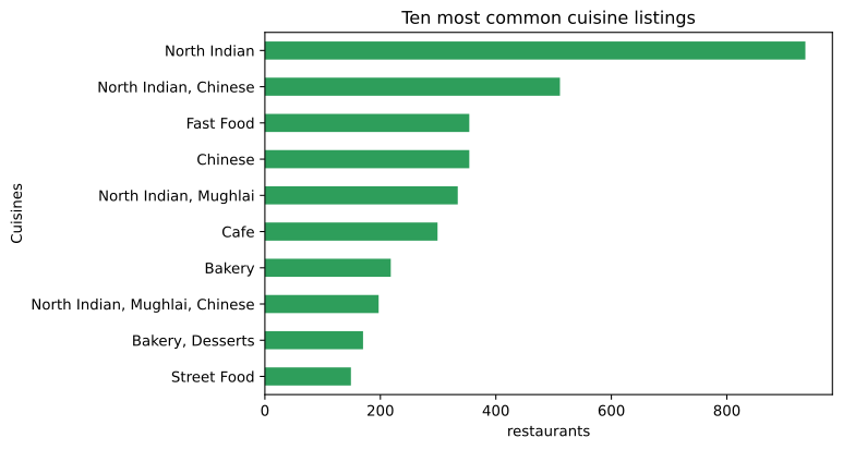
head(10) on the result keeps the ten biggest groups, and plot.barh() draws them as horizontal bars, which is the readable choice when the labels are long. sort_values() before plotting puts the biggest bar at the top, because a horizontal bar chart draws its first row at the bottom.
top = df['Cuisines'].value_counts().head(10)
print(top.to_string())

fig, ax = plt.subplots(figsize=(7, 4.5))
top.sort_values().plot.barh(ax=ax, color='#2e9e5b')
ax.set_xlabel('restaurants')
ax.set_title('Ten most common cuisine listings')
fig.savefig('chart.svg')Cuisines North Indian 936 North Indian, Chinese 511 Chinese 354 Fast Food 354 North Indian, Mughlai 334 Cafe 299 Bakery 218 North Indian, Mughlai, Chinese 197 Bakery, Desserts 170 Street Food 149
What the cuisine counts say
- North Indian alone is 936 restaurants, and it appears again inside three of the other nine listings. The column holds a comma separated list, not one category.
- 1,825 distinct listings over 9,551 rows means the top ten cover only a fifth of the table. A column like this needs splitting on the comma before it can be counted properly.
- Two listings tie at 354.
value_counts()keeps ties in the order it found them, so do not read the order of equal counts as a ranking.
The call that was removed
Older notebooks count through the top level function pd.value_counts(series) instead of the method. It was removed in pandas 2.2, and the attribute is gone, so the line fails at once rather than returning something wrong.
import pandas as pd

s = pd.Series(['India', 'India', 'UAE'])
pd.value_counts(s)Traceback (most recent call last):
File "main.py", line 4, in <module>
pd.value_counts(s)
AttributeError: module 'pandas' has no attribute 'value_counts'The fix is to call it on the Series: s.value_counts(). Every argument is the same.
value_counts vs groupby size
value_counts() | groupby(col).size() | |
|---|---|---|
| Works on | one Series | one or more columns of a frame |
| Order of the result | count, biggest first | the grouping values, sorted |
| Missing values | dropped unless dropna=False | dropped |
| Shares built in | yes, normalize=True | no, divide yourself |
| Use it for | a quick count of one column | a count across two columns, or a count plus another summary |
Where value_counts is the first call
- Checking a column's cardinality.
len(df[c].value_counts())says how many distinct values a column has, which decides how it can be encoded. - Finding the mode. The first index entry is the most frequent value, which is what Frequent category imputation fills with.
- Spotting a dirty level. Two spellings of one category show up as two rows with small counts, which no summary statistic would reveal.
value_counts() do not add up to len(df) when the column has missing values, because NaN is dropped by default. A percentage computed from those counts is a percentage of the non-missing rows. Pass dropna=False, or divide by len(df) yourself and say which denominator you used.Related
- Previous: One chart, one question, one observation
- Next: Pie and bar charts with a top-N trim
- See also: Frequent category imputation
- Reference: Series.value_counts in the pandas docs
- Run
df['City'].value_counts()and read how many distinct cities there are. - Add
sort=Falseto one of the calls and describe the order you get instead. - Count
df['Has Table booking']with and withoutnormalize=Trueand write the share of restaurants that take bookings.
You understood something today that you didn't yesterday.