
Dropping correlated features
Correlated features are two or more columns that move together closely enough to say the same thing, so keeping all of them adds cost and splits the credit for one effect.
Last updated: 12 Oct, 2026 · pandas 3.0 · scikit-learn 1.9
Dropping constant features removed columns that say nothing. This one removes columns that say something another column has already said. The Ames house price data is used throughout, because a house's garage size in cars and its garage size in square feet are the same fact written twice.
A note on a dataset you will meet in older material: load_boston was the usual example for this lesson and was removed from scikit-learn in version 1.2. Its B column encodes the proportion of Black residents per town as a feature assumed to affect house prices, and the maintainers removed the loader rather than keep shipping it. Importing it now raises ImportError with that reason. The Ames data makes the same point with no such problem.
Syntax: corr builds the square matrix of Pearson correlations between every pair of columns. numeric_only=True is required on a frame that has text columns, because the default tries to convert them and raises.
matrix = df.corr(numeric_only=True)   # one row and one column per numeric column
matrix.loc["GarageCars", "GarageArea"]
Finding the pairs that move together
Ranking every pair by correlation
A 36 by 36 matrix is 1296 numbers, most of them uninteresting. Taking the upper triangle and sorting by size turns it into a short list of pairs worth a decision.
import numpy as np

matrix = X.corr(numeric_only=True).abs()
upper = np.triu(np.ones(matrix.shape), 1).astype(bool)   # above the diagonal
pairs = matrix.where(upper).stack().sort_values(ascending=False)import numpy as np
import pandas as pd
AMES = ("https://raw.githubusercontent.com/krishnaik06/"
"Advanced-House-Price-Prediction-/master/train.csv")
df = pd.read_csv(AMES)
numeric = df.select_dtypes(include="number").drop(columns=["Id"])
X = numeric.drop(columns=["SalePrice"])
y = numeric["SalePrice"]
matrix = X.corr(numeric_only=True).abs()
upper = np.triu(np.ones(matrix.shape), 1).astype(bool)
pairs = matrix.where(upper).stack().sort_values(ascending=False)
print("numeric feature columns:", X.shape[1])
print()
print(pairs.head(8).round(4).to_string())numeric feature columns: 36 GarageCars GarageArea 0.8825 YearBuilt GarageYrBlt 0.8257 GrLivArea TotRmsAbvGrd 0.8255 TotalBsmtSF 1stFlrSF 0.8195 2ndFlrSF GrLivArea 0.6875 BedroomAbvGr TotRmsAbvGrd 0.6766 BsmtFinSF1 BsmtFullBath 0.6492 YearRemodAdd GarageYrBlt 0.6423
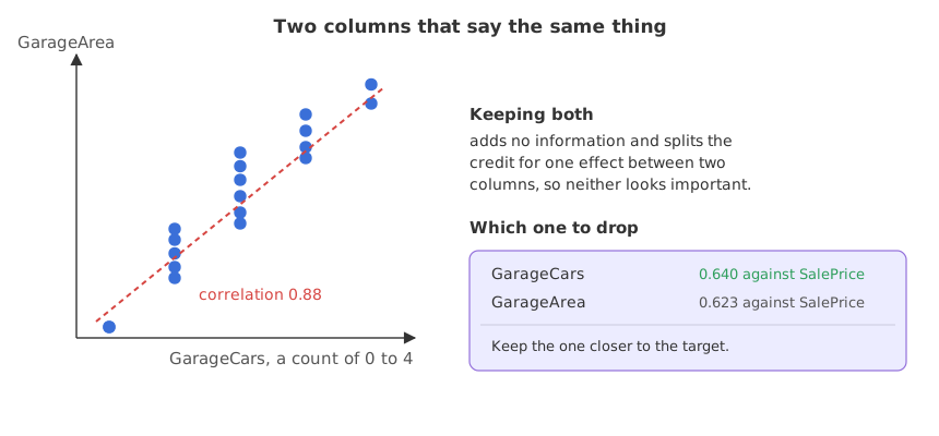
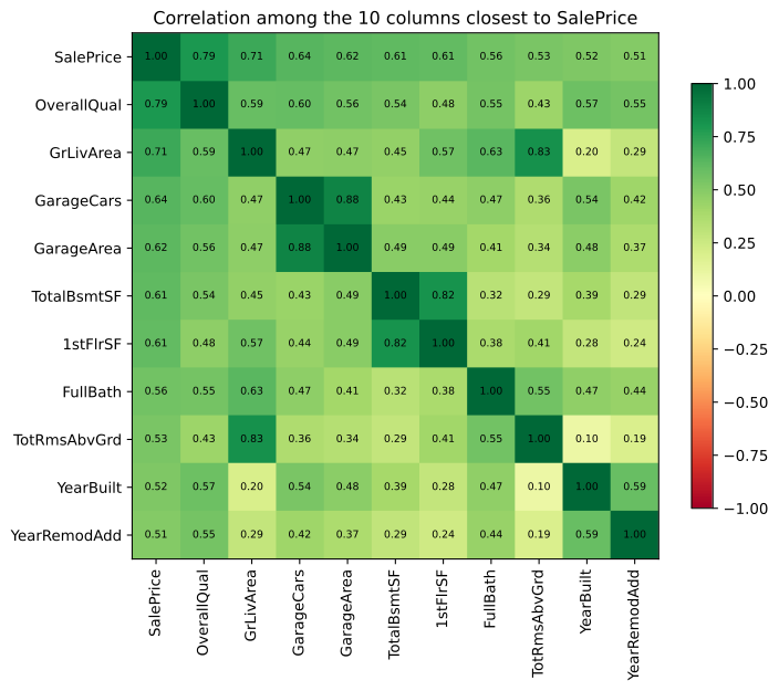
GarageCarsandGarageAreacorrelate at 0.88. One counts cars, the other measures square feet, and a bigger garage holds more cars.YearBuiltandGarageYrBltcorrelate at 0.83, because most garages were built with the house.GrLivAreaandTotRmsAbvGrdcorrelate at 0.83, andTotalBsmtSFand1stFlrSFat 0.82, which on a house with no second floor are nearly the same number.- Nothing reaches 0.95. On this data there is no pair where one column is a relabelled copy of another, which is common on raw data from a feed.
Seeing the matrix as a picture
A heatmap over all 36 columns is unreadable. Over the ten columns most closely related to the target it shows both the pairs to decide about and how each column relates to what is being predicted.
import matplotlib.pyplot as plt

top = numeric.corr(numeric_only=True)["SalePrice"].abs().sort_values(ascending=False).head(11)
block = numeric[top.index].corr(numeric_only=True)

fig, ax = plt.subplots(figsize=(8, 6.5))
image = ax.imshow(block, cmap="RdYlGn", vmin=-1, vmax=1)
ax.set_xticks(range(len(block)), block.columns, rotation=90)
ax.set_yticks(range(len(block)), block.columns)
for i in range(len(block)):
    for j in range(len(block)):
        ax.text(j, i, f"{block.iloc[i, j]:.2f}", ha="center", va="center", fontsize=7)
fig.colorbar(image, ax=ax, shrink=0.8)
ax.set_title("Correlation among the 10 columns closest to SalePrice")
plt.show()
print("columns drawn:", len(block))columns drawn: 11
Dropping one column from each pair
Collecting the columns to remove
Walking the lower triangle of the matrix and collecting the later column of every pair above the threshold gives a set of names to drop. The set takes care of a column that is correlated with several others, so it is only collected once.
def correlated_columns(frame, threshold):
    keep_out = set()
    matrix = frame.corr(numeric_only=True)
    for i in range(len(matrix.columns)):
        for j in range(i):                       # the lower triangle only
            if abs(matrix.iloc[i, j]) > threshold:
                keep_out.add(matrix.columns[i])  # drop the later of the pair
return keep_outdef correlated_columns(frame, threshold):
keep_out = set()
matrix = frame.corr(numeric_only=True)
for i in range(len(matrix.columns)):
for j in range(i): # the lower triangle only
if abs(matrix.iloc[i, j]) > threshold:
keep_out.add(matrix.columns[i]) # drop the later of the pair
return keep_out
for threshold in [0.9, 0.8, 0.7, 0.6]:
found = correlated_columns(X, threshold)
print(f"threshold {threshold}: {len(found)} columns -> {sorted(found)}")threshold 0.9: 0 columns -> [] threshold 0.8: 4 columns -> ['1stFlrSF', 'GarageArea', 'GarageYrBlt', 'TotRmsAbvGrd'] threshold 0.7: 4 columns -> ['1stFlrSF', 'GarageArea', 'GarageYrBlt', 'TotRmsAbvGrd'] threshold 0.6: 9 columns -> ['1stFlrSF', 'BsmtFullBath', 'FullBath', 'GarageArea', 'GarageCars', 'GarageYrBlt', 'GrLivArea', 'HalfBath', 'TotRmsAbvGrd']
- At 0.9 nothing is dropped, because no pair in this data is that close.
- At 0.8 four columns go, one from each of the four pairs above. 0.8 and 0.7 give the same answer, which is a sign the threshold is in a stable range.
- At 0.6 nine columns go, and the list now includes
GrLivAreaandGarageCars, two of the strongest predictors in the dataset. A threshold set too low removes signal, not duplication. - 0.8 to 0.9 is the usual range for this. Below 0.7 you are no longer removing duplicates.
Choosing which column of the pair to keep
The function above keeps whichever column appears first in the frame, which is an accident of column order. A better rule is to keep the one that correlates more strongly with the target, and that choice needs one extra line.
against_target = numeric.corr(numeric_only=True)["SalePrice"].abs()

for a, b in [("GarageCars", "GarageArea"), ("TotalBsmtSF", "1stFlrSF"),
             ("GrLivArea", "TotRmsAbvGrd"), ("YearBuilt", "GarageYrBlt")]:
    better = a if against_target[a] >= against_target[b] else b
    print(f"{a:14s} {against_target[a]:.4f}   {b:14s} {against_target[b]:.4f}"
f" keep {better}")GarageCars 0.6404 GarageArea 0.6234 keep GarageCars TotalBsmtSF 0.6136 1stFlrSF 0.6059 keep TotalBsmtSF GrLivArea 0.7086 TotRmsAbvGrd 0.5337 keep GrLivArea YearBuilt 0.5229 GarageYrBlt 0.4864 keep YearBuilt
On this dataset the two rules agree on every pair, because the stronger column happens to come first each time. That is luck, and it will not hold on a frame whose columns arrive in a different order. Judging against the target costs one line and removes the luck.
Dropping a correlated column against keeping both
| Drop one of the pair | Keep both | |
|---|---|---|
| Information lost | Almost none; the other column carries it | None |
| Linear model coefficients | Stable and readable | Shared between the two, and unstable from run to run |
| Tree model accuracy | Usually unchanged | Usually unchanged |
| Feature importance | One clear number | Split, so both look weaker than they are |
| Columns to collect in production | Fewer | More |
| Risk | Dropping the better of the two by accident | Carrying cost and confusing readers |
Where this check matters most
- Before a linear model. Two highly correlated columns make the coefficients unstable and their signs unreliable, which is the problem known as multicollinearity.
- Before explaining a model. Split importance makes a strong feature look weak, and someone will draw the wrong conclusion from the chart.
- After joining tables. A join is where exact duplicates appear, under two different names, with a correlation of 1.0.
df.corr() without numeric_only=True raises ValueError: could not convert string to float: 'RL' on any frame with a text column. Pearson correlation also only finds straight-line relationships: two columns can move together perfectly and still correlate at zero, which is what Mutual information picks up.Related
- Previous: Dropping constant features
- Next: Mutual information
- See also: Relationships between features
- Reference: DataFrame.corr in the pandas API reference
- Pass
method="spearman"tocorrin the helper and compare the list at 0.8; Spearman ranks the values first, so it catches curved relationships Pearson misses. - Rewrite
correlated_columnsso it drops whichever column of the pair has the weaker correlation withSalePrice, and check that it still returns four names at 0.8. - Fit a
LinearRegressiononGarageCarsandGarageAreatogether, print the two coefficients, then fit on each alone and compare.
This is what real progress feels like.