
Log, reciprocal and square root transformations
A Gaussian transformation is a function applied to one column, such as a logarithm or a square root, that pulls a skewed distribution closer to a normal one.
Last updated: 12 Oct, 2026 · pandas 3.0 · scikit-learn 1.9 · scipy 1.18
Reading a Q-Q plot gave the measuring instrument. Four transformations are written by hand below, applied to one column, and read off the chart after each one. There is no best transformation: which one wins depends on the data, so the method is to try them all and keep the straightest Q-Q plot.
Which models assume a normal column
- Linear and logistic regression are derived under the assumption that the inputs, and more importantly the errors, are normally distributed. They still run without it and usually fit better with it.
- Anything that uses a mean and a standard deviation to describe a column, which includes standardisation itself and Gaussian naive Bayes.
- Trees need none of this. A monotonic function of a column leaves every split available, so a log transform changes a tree's answer no more than a scaler does.
The four transformations
Each one is a single expression over the column. Three of them have a constraint, which is the thing to check before applying them.
import numpy as np

log_age = np.log(age)            # undefined at 0, and negative values give NaN
recip_age = 1 / age              # undefined at 0
sqrt_age = age ** 0.5            # negative values give NaN
power_age = age ** (1 / 1.2)     # a power transform; the exponent is yours to choose
The last line raises each value to a fractional power. Any exponent below 1 pulls a long right tail in, and the closer it is to 1 the gentler the pull; 1/2 is the square root and 1/1.2 is a weaker version of it. The video calls this one an exponential transformation; the name for raising a value to a fixed power is a power transform, and an exponential transformation is the other way round, a fixed base raised to the value.
Ranking the four on Titanic Age
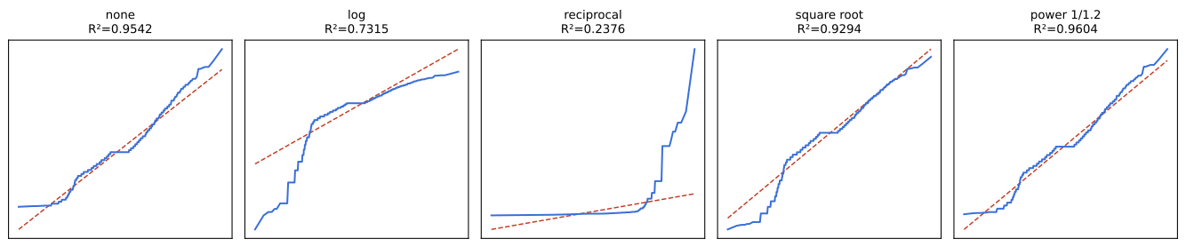
Age is the column the video works through. Running all five candidates, the untransformed column included, and reading R² off each Q-Q plot turns the choice into a comparison rather than a judgement.
import pandas as pd

URL = "https://raw.githubusercontent.com/krishnaik06/Feature-Engineering-Live-sessions/master/titanic.csv"
df = pd.read_csv(URL, usecols=['Age', 'Fare'])
df['Age'] = df['Age'].fillna(df['Age'].median()) # 177 missing ages, filled with 28.0def fit(values):
# the correlation probplot already computes, squared
(_, _), (_, _, r) = stats.probplot(np.asarray(values), dist='norm')
return r ** 2import matplotlib.pyplot as plt
import numpy as np
import scipy.stats as stats
def fit(values):
    # the correlation probplot already computes, squared
    (_, _), (_, _, r) = stats.probplot(np.asarray(values), dist='norm')
    return r ** 2
age = df['Age']
candidates = [('none', age), ('log', np.log(age)), ('reciprocal', 1 / age),
('square root', age ** 0.5), ('power 1/1.2', age ** (1 / 1.2))]
fig, ax = plt.subplots(1, 5, figsize=(14, 3.0))
for a, (name, values) in zip(ax, candidates):
(osm, osr), (slope, intercept, r) = stats.probplot(np.asarray(values), dist='norm')
a.plot(osm, slope * osm + intercept, color='#c23b22', lw=1.1, ls='--')
a.plot(osm, osr, color='#3a6fd8', lw=1.5)
a.set_title(f'{name}\nR²={r ** 2:.4f}', fontsize=10)
a.set_xticks([]); a.set_yticks([])
print(f"{name:12s} skew {stats.skew(values):7.3f} R² {fit(values):.4f}")
fig.tight_layout()none skew 0.509 R² 0.9542 log skew -2.655 R² 0.7315 reciprocal skew 7.608 R² 0.2376 square root skew -0.758 R² 0.9294 power 1/1.2 skew 0.148 R² 0.9604
Reading the five scores
- power 1/1.2 wins at 0.9604, with a skew of 0.148, the closest to zero of the five.
- Doing nothing scores 0.9542. Age was already close to normal, so the gain from the best transformation is small. That is a real answer: leaving a column alone is a choice worth measuring.
- log drops to 0.7315 and its skew swings to −2.655. A logarithm pulls the right tail in hard, and on a column that was barely skewed it overshoots into a left tail.
- reciprocal is the worst at 0.2376. It turns small ages into very large numbers, so the children dominate.
- square root scores 0.9294, between the log and the gentler power.
The column where a logarithm is the right answer
Fare is the skewed column, and it is also the one where np.log has a problem: 15 passengers paid nothing. The logarithm of 0 is minus infinity, and numpy returns that instead of raising, so the failure is silent until a later step gives nonsense.
import numpy as np
import scipy.stats as stats

logged = np.log(df['Fare'])
print("zero fares in the column:", int((df["Fare"] == 0).sum()))
print("smallest logged value   :", logged.min())
print("infinite values          :", int(np.isinf(logged).sum()))
(_, _), (_, _, r) = stats.probplot(np.asarray(logged), dist='norm')
print("R² of the Q-Q line :", r ** 2)zero fares in the column: 15 smallest logged value : -inf infinite values : 15 R² of the Q-Q line : nan
- 15 fares are 0. Those are the free passages in the Titanic manifest.
- The smallest logged value is
-inf. numpy prints a runtime warning and carries on. - R² comes back as
nan. Nothing raised, the chart is empty, and a reader who only looked at the chart would see a blank panel and wonder why.
log1p, which is log of one plus the value
np.log1p(x) computes log(1 + x). The shift of one puts every value above zero, so a column that reaches down to 0 survives, and the accuracy for tiny values is better than writing np.log(x + 1) by hand. np.expm1 is the inverse, which matters when a transformed target has to be read back in real units.
import matplotlib.pyplot as plt
import numpy as np
import scipy.stats as stats

fare = df['Fare']
fixed = np.log1p(fare)                     # log(1 + x), safe at x = 0

fig, ax = plt.subplots(1, 2, figsize=(9, 3.4))
for a, values, name in [(ax[0], fare, 'Fare'), (ax[1], fixed, 'np.log1p(Fare)')]:
    (osm, osr), (slope, intercept, r) = stats.probplot(np.asarray(values), dist='norm')
    a.plot(osm, slope * osm + intercept, color='#c23b22', lw=1.1, ls='--')
    a.plot(osm, osr, color='#3a6fd8', lw=1.6)
    a.set_title(f'{name}  R²={r ** 2:.4f}', fontsize=10)
    a.set_xlabel('normal quantiles')
    print(f"{name:16s} skew {stats.skew(values):7.3f}   R² {r ** 2:.4f}")
fig.tight_layout()
print("smallest value after log1p:", round(float(fixed.min()), 4))
print("back to fares again :", np.expm1(fixed).head(3).round(4).tolist())Fare skew 4.779 R² 0.5190 np.log1p(Fare) skew 0.394 R² 0.9150 smallest value after log1p: 0.0 back to fares again : [7.25, 71.2833, 7.925]
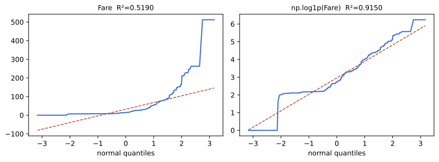
- Skew falls from 4.779 to 0.394 and R² rises from 0.5190 to 0.9150. The same column, one function applied.
- The smallest value is 0.0, which is log(1 + 0), so the zero fares came through without a warning.
np.expm1gives the original fares back, which is how a prediction made on a transformed target is reported in rupees or pounds rather than in logs.
Choosing between the transformations
| Transformation | Expression | Constraint | Pulls in |
|---|---|---|---|
| Logarithm | np.log(x) | x > 0 strictly | a long right tail, hard |
| log of one plus x | np.log1p(x) | x > −1 | a long right tail, hard, and survives zeros |
| Reciprocal | 1 / x | x ≠ 0 | reverses the order of the column |
| Square root | x ** 0.5 | x ≥ 0 | a right tail, gently |
| Power | x ** (1 / k) | x ≥ 0 for a fractional power | a right tail, as gently as k allows |
Where these transformations are used
- Money and counts. Prices, incomes, page views and claim sizes are nearly always right skewed, and log1p is the usual first try.
- The target of a regression, not only its inputs. A log transformed target is often what turns a poor fit into a good one, and the prediction is read back with
np.expm1. - Before a model that assumes normality, which is linear regression, logistic regression and Gaussian naive Bayes.
np.log(0) gives -inf and a runtime warning, not an exception, and np.log(-1) gives nan the same way. Every later step then quietly produces nan. Check the minimum of a column before taking its logarithm, and use np.log1p whenever zero is a legal value.Related
- Previous: Reading a Q-Q plot
- Next: Box-Cox and Yeo-Johnson
- See also: Standardisation
- Reference: numpy.log1p in the NumPy docs
- Change the exponent from
1 / 1.2to1 / 1.5and to1 / 1.05. Watch R² rise and then fall; there is a best exponent in between, which is what the Box-Cox search finds without guessing. - Apply
np.log1pto Age and compare it with the power transform. The gentler transformation wins on a column that was barely skewed. - Replace the 15 zero fares with the smallest non zero fare, then take a plain
np.log. The warning disappears and R² becomes a real number.
Little by little, you're building something great.