
Min max scaling
Min max scaling rewrites a column as (x − minimum) / (maximum − minimum), so every value lands between 0 and 1.
Last updated: 12 Oct, 2026 · pandas 3.0 · scikit-learn 1.9 · scipy 1.18
Standardisation centred each column at zero and left its range open. Min max scaling fixes the range instead and lets the centre fall where it may. It is the scaling used on image pixels, where dividing by 255 is this formula with a minimum of 0.
Syntax: the same three calls as every scaler, with a feature_range argument if 0 to 1 is not what you want.
from sklearn.preprocessing import MinMaxScaler

scaler = MinMaxScaler()              # feature_range=(0, 1) by default
out = scaler.fit_transform(df)
Scaling the four Titanic columns
The same four columns as before, with the median filled into Age, so the two scalers can be compared row for row.
import pandas as pd

URL = "https://raw.githubusercontent.com/krishnaik06/Feature-Engineering-Live-sessions/master/titanic.csv"
df = pd.read_csv(URL, usecols=['Survived', 'Pclass', 'Age', 'Fare'])
df['Age'] = df['Age'].fillna(df['Age'].median()) # 177 missing ages, filled with 28.0from sklearn.preprocessing import MinMaxScaler
scaler = MinMaxScaler().set_output(transform='pandas')
scaled = scaler.fit_transform(df)Putting every column between 0 and 1
from sklearn.preprocessing import MinMaxScaler

scaler = MinMaxScaler().set_output(transform='pandas')
scaled = scaler.fit_transform(df)
print(scaled.head(3).round(6).to_string())
print("\nmin:", scaled.min().tolist())
print("max:", scaled.max().tolist())
print("\nlearned data_min_:", scaler.data_min_.tolist())
print("learned data_max_:", scaler.data_max_.tolist())
low, high = scaler.data_min_[2], scaler.data_max_[2]
print("first age by hand:", round((df.loc[0, "Age"] - low) / (high - low), 6))Survived Pclass Age Fare 0 0.0 1.0 0.271174 0.014151 1 1.0 0.0 0.472229 0.139136 2 1.0 1.0 0.321438 0.015469 min: [0.0, 0.0, 0.0, 0.0] max: [1.0, 1.0, 1.0, 1.0] learned data_min_: [0.0, 1.0, 0.42, 0.0] learned data_max_: [1.0, 3.0, 80.0, 512.3292] first age by hand: 0.271174
Reading the scaled columns
- Every column runs from 0.0 to 1.0 exactly. That is guaranteed on the data the scaler was fitted on, and only on that data.
data_min_anddata_max_are what it learned: the smallest and largest value of each column, 0.42 and 80.0 for Age.- The first fare is 0.014151, which says that a fare of 7.25 sits one and a half percent of the way from the cheapest ticket to the most expensive one.
- Pclass comes through as 0, 0.5 and 1, and Survived as 0 and 1. A column with three levels gets three evenly spaced values, which is worth noticing before an already encoded category is handed to a scaler.
Where the extreme fare sends the rest
One passenger paid 512.33 while the median fare is 14.45. That single value sets data_max_, and every other fare is measured against it.
import matplotlib.pyplot as plt

fig, ax = plt.subplots(1, 2, figsize=(9, 3.4))
ax[0].hist(scaled["Age"], bins=20, color="#3a6fd8")
ax[0].set_title("Age after min max scaling")
ax[1].hist(scaled["Fare"], bins=20, color="#d8733a")
ax[1].set_title("Fare after min max scaling")
for a in ax:
    a.set_xlabel("scaled value"); a.set_ylabel("passengers")
fig.tight_layout()

print("median fare lands at :", round(scaled["Fare"].median(), 4))
print("share of fares below 0.1:", f"{(scaled['Fare'] < 0.1).mean():.1%}")
print("median age lands at :", round(scaled["Age"].median(), 4))median fare lands at : 0.0282 share of fares below 0.1: 82.2% median age lands at : 0.3466
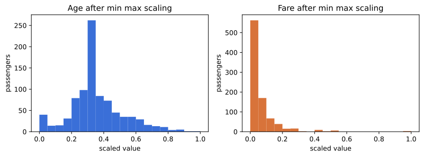
- The median fare lands at 0.0282. Half the passengers sit in the bottom three percent of the scaled range, because the range belongs to one ticket.
- 82.2% of fares fall below 0.1. The transform did what it promised and still left the column unusable for anything that compares distances.
- Age is unaffected because it has no such extreme. Min max scaling is only as good as the two values it learns.
Min max scaling compared with standardisation
| MinMaxScaler | StandardScaler | |
|---|---|---|
| Formula | (x − min) / (max − min) | (x − mean) / standard deviation |
| Output range | 0 to 1, guaranteed on the fitted data | open, usually about −3 to 3 |
| Learns | the minimum and the maximum | the mean and the standard deviation |
| Effect of one extreme value | sets the whole range, squeezes everything else | moves the mean and the standard deviation a little |
| New value outside the fitted range | goes below 0 or above 1 | goes further from 0, nothing special happens |
| Usual home | image pixels, neural network inputs | most other models |
Where min max scaling is used
- Image pixels. Values arrive as 0 to 255 and are divided by 255, which is this formula with a minimum of 0 and a maximum of 255.
- Neural network inputs, where a bounded input range keeps the first layer's activations in a sensible place.
- Anything that must be read as a proportion, such as a score shown to a user as a percentage of the observed range.
Related
- Previous: Standardisation
- Next: Robust scaling
- See also: Why features are scaled
- Reference: MinMaxScaler in the scikit-learn docs
- Pass
feature_range=(-1, 1)and read the minimum and maximum again. - Transform a one row frame with a fare of 600 using the fitted scaler. The result is larger than 1.
- Drop the one passenger who paid 512.33 before fitting, then look at where the median fare lands. It moves a long way up.
Slow is fine. Stopping is the only problem.