
Model based selection with Lasso
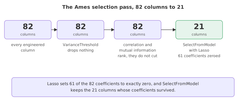
Model based selection lets a fitted model decide which columns matter: Lasso drives the coefficients of useless columns to exactly zero, and SelectFromModel keeps the columns whose coefficients survived.
Last updated: 12 Oct, 2026 · pandas 3.0 · scikit-learn 1.9
Every filter so far scored each column on its own. Mutual information cannot tell that two columns say the same thing, and Chi square for categorical features cannot tell that a column only matters alongside another. A model fitted on all the columns at once sees both.
Ordinary least squares picks coefficients that make the squared error as small as possible. Lasso adds a penalty equal to alpha times the sum of the absolute coefficients. Because the penalty on a coefficient is a straight line through zero rather than a curve, the cheapest answer for a column that is not pulling its weight is a coefficient of exactly 0, not merely a small one. That is what makes Lasso a selector, and ridge regression, whose penalty squares the coefficients instead, not one: ridge shrinks a coefficient towards zero without ever reaching it.
Syntax: SelectFromModel wraps any estimator that exposes coef_ or feature_importances_ after fitting.
from sklearn.linear_model import Lasso
from sklearn.feature_selection import SelectFromModel

selector = SelectFromModel(Lasso(alpha=0.005, random_state=0))
selector.fit(X, y)              # fits the Lasso, then reads its coefficients
selector.get_support()          # True for every column whose coefficient is not zero
selector.estimator_.coef_       # the fitted Lasso's coefficients
Preparing the 82 columns
Lasso needs numbers, no missing values and columns on a comparable scale, because a single alpha penalises every coefficient equally and a coefficient's size depends on its column's units. The steps below are the ones the earlier parts covered, applied in order to the Ames data.
Loading and splitting the columns by type
pd.api.types.is_string_dtype is the test that works on pandas 3. The older df[c].dtypes == 'O' returns False for every column now, which silently puts all 43 text columns into the numeric list.
import numpy as np
import pandas as pd

AMES = ("https://raw.githubusercontent.com/krishnaik06/"
        "Advanced-House-Price-Prediction-/master/train.csv")
df = pd.read_csv(AMES)

text = [c for c in df.columns if pd.api.types.is_string_dtype(df[c])]
numeric = [c for c in df.columns if c not in text]
Filling the missing values
Text columns get the label "Missing". Numeric columns get the median, plus an extra 0 or 1 column recording that the value was absent, which is often informative on its own. Those extra columns are why 81 becomes 84 before the id and the target come out.
text_nan = [c for c in text if df[c].isnull().sum() > 1]
df[text_nan] = df[text_nan].fillna("Missing")

numeric_nan = [c for c in numeric if df[c].isnull().sum() > 1]
for c in numeric_nan:
    df[c + "nan"] = np.where(df[c].isnull(), 1, 0)   # keep the fact it was missing
    df[c] = df[c].fillna(df[c].median())             # assignment, not inplace
Turning years into ages and skew into logs
A year of construction is only useful relative to the year of sale, so the difference replaces it. The four skewed size columns and the target are logged, which pulls their long right tails in.
for c in ["YearBuilt", "YearRemodAdd", "GarageYrBlt"]:
    df[c] = df["YrSold"] - df[c]           # a year becomes an age

for c in ["LotFrontage", "LotArea", "1stFlrSF", "GrLivArea", "SalePrice"]:
    df[c] = np.log(df[c])                  # the skewed columns and the target
Grouping rare labels, then encoding by the target
Any label in fewer than 1 per cent of rows becomes Rare_var, so a category seen twice does not get a code of its own. Each text column is then replaced by an integer that follows the mean price of its labels, lowest to highest. That ordering is computed from the target, so it is the step with the most to gain from being cross-fitted; Mean encoding measures what the naive form memorises and shows the TargetEncoder version that cures it.
for c in text:
    share = df.groupby(c)["SalePrice"].count() / len(df)
    common = share[share > 0.01].index                     # labels in over 1% of rows
    df[c] = np.where(df[c].isin(common), df[c], "Rare_var")

for c in text:
    order = df.groupby(c)["SalePrice"].mean().sort_values().index
    df[c] = df[c].map({k: i for i, k in enumerate(order, 0)})
Scaling into 0 to 1
MinMaxScaler maps every column into 0 to 1, so one alpha means the same thing for a column of square feet and a column holding a code from 0 to 4.
from sklearn.preprocessing import MinMaxScaler

features = [c for c in df.columns if c not in ["Id", "SalePrice"]]
X = pd.DataFrame(MinMaxScaler().fit_transform(df[features]), columns=features)
y = df["SalePrice"]
Letting Lasso make the cut
import numpy as np
from sklearn.linear_model import Lasso
from sklearn.feature_selection import SelectFromModel

selector = SelectFromModel(Lasso(alpha=0.005, random_state=0))
selector.fit(X, y)
selected = X.columns[selector.get_support()]

print("total features:   ", X.shape[1])
print("selected features:", len(selected))
print("coefficients shrunk to zero:", int(np.sum(selector.estimator_.coef_ == 0)))
print()
print(list(selected))total features: 82 selected features: 21 coefficients shrunk to zero: 61 ['MSSubClass', 'MSZoning', 'Neighborhood', 'OverallQual', 'YearRemodAdd', 'RoofStyle', 'BsmtQual', 'BsmtExposure', 'HeatingQC', 'CentralAir', '1stFlrSF', 'GrLivArea', 'BsmtFullBath', 'KitchenQual', 'Fireplaces', 'FireplaceQu', 'GarageType', 'GarageFinish', 'GarageCars', 'PavedDrive', 'SaleCondition']
- 82 columns went in and 21 came out. Three quarters of the frame was dropped by one fit.
- 61 coefficients are exactly 0, and 21 plus 61 is 82, so every column is accounted for.
SelectFromModelmade no separate decision: it kept whatever Lasso did not zero. - The survivors read like a valuer's list. Overall quality, living area, first floor area, kitchen quality, the garage, the neighbourhood and the fireplaces.
- The survivors include
1stFlrSFandGarageCarsbut notGarageArea,TotalBsmtSForTotRmsAbvGrd. Lasso settles the correlated pairs from Dropping correlated features by keeping one of each, and it decides which one from the whole fit rather than from a threshold applied to one pair at a time.
What alpha controls
alpha is the strength of the penalty, and it is the only dial on this method. The bigger it is, the more coefficients are pushed to zero and the fewer columns survive.
from sklearn.linear_model import Lasso

for alpha in [0.001, 0.002, 0.005, 0.01, 0.02, 0.05]:
    model = Lasso(alpha=alpha, random_state=0).fit(X, y)
print(f"alpha {alpha:<6} columns kept {int((model.coef_ != 0).sum()):3d}")alpha 0.001 columns kept 41 alpha 0.002 columns kept 33 alpha 0.005 columns kept 21 alpha 0.01 columns kept 13 alpha 0.02 columns kept 8 alpha 0.05 columns kept 3
The count falls steeply, so alpha should be chosen by cross-validation against the score you care about rather than picked by eye. LassoCV does exactly that and reports the alpha it chose in alpha_.
Reading the coefficients that survived
A Lasso coefficient on scaled columns is directly comparable with the others, because every column spans the same 0 to 1 range. That makes the fitted model an explanation as well as a selector.
import pandas as pd
from sklearn.linear_model import Lasso
from sklearn.feature_selection import SelectFromModel

selector = SelectFromModel(Lasso(alpha=0.005, random_state=0)).fit(X, y)
coefficients = pd.Series(selector.estimator_.coef_, index=X.columns)
survivors = coefficients[coefficients != 0].sort_values(key=abs, ascending=False)

print(survivors.head(8).round(4).to_string())
print()
print("negative coefficients:", int((survivors < 0).sum()))GrLivArea 0.7345 OverallQual 0.4492 Neighborhood 0.3264 GarageCars 0.1666 KitchenQual 0.1240 1stFlrSF 0.1048 YearRemodAdd -0.0929 FireplaceQu 0.0812 negative coefficients: 2
GrLivAreahas the largest coefficient, and the target is a log price, so the coefficient is a proportional effect rather than a number of dollars.YearRemodAddis negative, which is correct after the year was turned into an age: more years since the remodel means a lower price.- The ranking here and the mutual information ranking agree at the top and diverge below it, because this one accounts for what the other columns already explain.
Filter methods against model based selection
| Filter (variance, correlation, chi square, mutual information) | Embedded (SelectFromModel) | |
|---|---|---|
| Sees columns | One at a time | All at once |
| Handles duplicates | No, both copies score the same | Yes, one of the pair is zeroed |
| Needs a model | No | Yes, and the choice suits that model |
| Cost | One pass over the data | One model fit |
| How many to keep | You choose k or a percentile | The penalty decides |
| Risk | Keeping redundant columns | A choice tied to one estimator and one alpha |
Where this is the method to reach for
- After the cheap filters. Drop the constant and the duplicated columns first, then let a model settle what is left; a fit on 82 columns is faster and steadier than one on 500.
- When the model is linear anyway. A Lasso selection followed by a linear model is coherent, because the selection used the same notion of usefulness as the final fit.
- When the column list has to be defended. A coefficient of exactly zero is a cleaner answer than a score that fell below an arbitrary cut.
SelectFromModel is fitted here on the whole dataset so the numbers can be compared with the engineering steps above. In a real run the whole sequence, the imputation, the target encoding, the scaler and the selector, is fitted on the training rows only and applied to the test rows. Otherwise the 21 columns were chosen with the test set's help, and every score measured afterwards is flattered. The target encoding above is the step that leaks hardest, which is why Mean encoding cross-fits it. Pipelines and pandas output makes that one object. Lasso also requires scaled columns: run it on raw square feet beside a 0 to 4 code and the penalty falls almost entirely on the small column.Related
- Previous: Chi square for categorical features
- Next: Data leakage
- See also: Project: the feature selection
- Reference: SelectFromModel and Lasso in the scikit-learn user guide
- Replace
LassowithRandomForestRegressor(n_estimators=100, random_state=0)insideSelectFromModeland compare the two lists; the forest selects on importance above the mean rather than on a zero coefficient. - Pass
threshold="median"toSelectFromModeland printget_support().sum(). All 82 survive, because 61 coefficients are 0, so the median absolute coefficient is 0 and every column clears it. - Fit
LassoCV(cv=5, random_state=0)on the same frame and printalpha_and how many coefficients it left non-zero.
You understood something today that you didn't yesterday.