
Chi square for categorical features
The chi square test scores a feature by how far the counts it produces per class sit from the counts expected if the feature and the target were unrelated.
Last updated: 12 Oct, 2026 · pandas 3.0 · scikit-learn 1.9
Mutual information ranked columns by dependence of any kind. Chi square answers a narrower question with a statistical test behind it, and it is the standard filter for counts and categories.
The idea is a table. For each value of the feature and each class of the target, count the rows. Then work out what each count would be if the two were independent, which is the row total times the column total divided by the grand total. The statistic adds up (observed - expected)^2 / expected over every cell. A large value means the counts could not plausibly have come from an unrelated pair.
Syntax: chi2 returns two arrays, the statistic per column and the p value per column.
from sklearn.feature_selection import chi2, SelectKBest

statistic, p_value = chi2(X, y)                  # X must be non-negative
SelectKBest(score_func=chi2, k=10).fit(X, y)     # the same score, as a transformer
Scoring the mobile price columns
The mobile price dataset has 2000 phones, 20 columns describing each and a target with four price bands of 500 phones each. Every column is a non-negative count or measurement, which is what chi square needs.
import pandas as pd

MOBILE = ("https://raw.githubusercontent.com/krishnaik06/"
          "Feature-Engineering-Live-sessions/master/mobile_dataset.csv")
df = pd.read_csv(MOBILE)

X = df.drop(columns="price_range")
y = df["price_range"]import pandas as pd
MOBILE = ("https://raw.githubusercontent.com/krishnaik06/"
"Feature-Engineering-Live-sessions/master/mobile_dataset.csv")
df = pd.read_csv(MOBILE)
X = df.drop(columns="price_range")
y = df["price_range"]
from sklearn.feature_selection import chi2
statistic, p_value = chi2(X, y)
table = pd.DataFrame({"feature": X.columns, "chi2": statistic, "p": p_value})
table = table.sort_values("chi2", ascending=False)
print(table.head(8).to_string(index=False))
print()
print(table.tail(4).to_string(index=False)) feature chi2 p
ram 931267.519053 0.000000e+00
px_height 17363.569536 0.000000e+00
battery_power 14129.866576 0.000000e+00
px_width 9810.586750 0.000000e+00
mobile_wt 95.972863 1.140850e-20
int_memory 89.839124 2.371978e-19
sc_w 16.480319 9.037659e-04
talk_time 13.236400 4.152292e-03
feature chi2 p
clock_speed 0.648366 0.885276
dual_sim 0.631011 0.889298
wifi 0.422091 0.935642
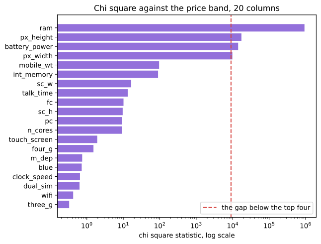
three_g 0.327643 0.954748ramscores 931267.5, about fifty times the next column. Memory size decides a phone's price band almost on its own.- Four columns clear 9000, and all four are physical quantities: memory, screen pixels and battery capacity.
- The p values for those four print as 0.0. They are smaller than the smallest number a float can hold, which is not a bug but a sign the statistic is enormous.
- The bottom of the table is near zero.
three_gscores 0.33 at a p value of 0.95, so the counts are what you would expect if the column and the price band had nothing to do with each other. - The scale is not comparable across column types.
ramruns to 4000 andblueis 0 or 1, and chi square grows with the size of the counts, so the ranking is more trustworthy than the gaps between the numbers.
The scores span six orders of magnitude, so a log scale is the only way to see them all at once.
import matplotlib.pyplot as plt

ordered = table.sort_values("chi2")

plt.figure(figsize=(7, 5.5))
plt.barh(range(len(ordered)), ordered["chi2"], color="#9370DB")
plt.yticks(range(len(ordered)), ordered["feature"])
plt.xscale("log")
plt.axvline(9000, color="#d64541", linestyle="--", label="the gap below the top four")
plt.xlabel("chi square statistic, log scale")
plt.title("Chi square against the price band, 20 columns")
plt.legend(loc="lower right")
plt.show()
print("largest / smallest:", round(ordered["chi2"].max() / ordered["chi2"].min()))largest / smallest: 2842326
Keeping the best k columns
SelectKBest wraps the same score and returns a transformer, which is what goes into a pipeline. k is the number of columns to keep.
from sklearn.feature_selection import chi2, SelectKBest

selector = SelectKBest(score_func=chi2, k=10).fit(X, y)
kept = list(X.columns[selector.get_support()])

print("kept:   ", kept)
print("dropped:", [c for c in X.columns if c not in kept])
print()
print("shape in: ", X.shape, " shape out:", selector.transform(X).shape)kept: ['battery_power', 'fc', 'int_memory', 'mobile_wt', 'px_height', 'px_width', 'ram', 'sc_h', 'sc_w', 'talk_time'] dropped: ['blue', 'clock_speed', 'dual_sim', 'four_g', 'm_dep', 'n_cores', 'pc', 'three_g', 'touch_screen', 'wifi'] shape in: (2000, 20) shape out: (2000, 10)
Six of the ten dropped columns are yes-or-no flags: blue, dual_sim, four_g, three_g, touch_screen and wifi. The other four hold small numbers: clock_speed, m_dep, n_cores and pc. On this dataset the price band is decided by what the hardware measures, not by which features are present.
The non-negative rule, and what breaks it
Chi square compares observed counts with expected counts, and a count cannot be negative. scikit-learn enforces this. Scaling a frame with StandardScaler, which centres every column on zero, makes half the values negative and breaks the test.
from sklearn.preprocessing import StandardScaler
from sklearn.feature_selection import chi2

X_scaled = StandardScaler().fit_transform(X)
chi2(X_scaled, y)Traceback (most recent call last):
File "main.py", line 5, in <module>
chi2(X_scaled, y)
ValueError: Input X must be non-negative.- The error names the rule exactly. There is no warning and no partial result.
MinMaxScaleris the scaler that works here, because it maps every column into 0 to 1 and leaves nothing negative.- Chi square needs no scaling at all when the columns are already counts, which is the usual case for it.
Chi square against mutual information
| Chi square | Mutual information | |
|---|---|---|
| Target type | Classes only | Classes or a continuous value |
| Feature values | Non-negative only | Anything |
| Returns | A statistic and a p value | A score with no significance test |
| Reproducible | Exactly; it has no random step | Only with random_state= |
Reads a quantity like ram | As counts, so a large column scores large | On its information, whatever its scale |
| Best for | Counts, flags and encoded categories | Mixed columns and odd relationships |
Where chi square fits
- Text classification. A bag of words frame is non-negative counts against a class label, which is exactly the shape chi square was made for.
- One hot encoded categories. Each dummy is 0 or 1 and non-negative, so the test asks whether a label and a class occur together more often than chance.
- Survey and questionnaire data. Counts per answer per group is the textbook contingency table.
Related
- Previous: Mutual information
- Next: Model based selection with Lasso
- See also: Why features are dropped
- Reference: chi2 in the scikit-learn API reference
- Change
kto 4 and print what survives; compare it with the four columns whose p value printed as 0.0. - Run
chi2onMinMaxScaler().fit_transform(X)and compare the ranking with the unscaled one; the same four columns lead, in a different order, which is how much the raw size of a column moves the statistic. - Split the data first with
train_test_split(..., random_state=0, stratify=y), score only the training half and check thatramstill leads.
Little by little, you're building something great.