
Project: the house price data
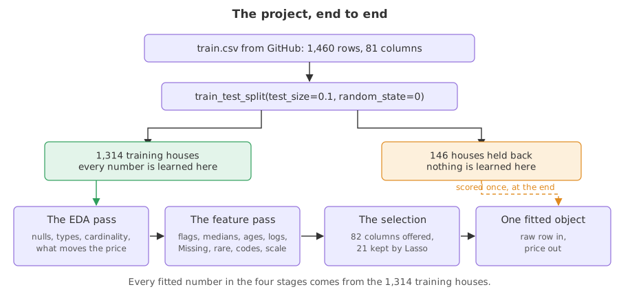
The house price project is one dataset carried from a raw CSV to a single fitted object: 1,460 house sales in Ames, Iowa, described by 81 columns, with a sale price to predict.
Last updated: 12 Oct, 2026 · pandas 3.0 · scikit-learn 1.9
Everything so far was shown on one technique at a time. The five lessons of this project use one table and keep going: look at it, build features from it, cut those features down and end with an object that takes a raw row and returns a price. Pipelines and pandas output built the container; this is what goes in it.
Reading the file and naming the target
The file is read straight from its raw GitHub address, so there is nothing to download. SalePrice is the target; Id is a row number with no meaning, so it leaves with the target.
AMES = ("https://raw.githubusercontent.com/krishnaik06/"
        "Advanced-House-Price-Prediction-/master/train.csv")
houses = pd.read_csv(AMES)      # (1460, 81)
X = houses.drop(columns=['Id', 'SalePrice'])
Taking the log of the price
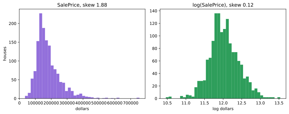
House prices are right skewed: most houses cluster low and a few expensive ones stretch the tail. A linear model fitted on that chases the tail. Taking the natural log pulls it in, and because every price is above zero the log is defined for every row. Log, reciprocal and square root transformations covers what the transform does to a column.
y = np.log(houses['SalePrice'])   # the model predicts a log price
# np.exp(prediction) turns it back into dollars at the end
Splitting before anything else
The split is the first operation, not the last. Ten percent is held back, which leaves 1,314 houses to learn from and 146 to be scored on once. random_state=0 makes the same split come back tomorrow.
X_train, X_test, y_train, y_test = train_test_split(
    X, y, test_size=0.1, random_state=0)
Loading, describing and splitting in one run
import numpy as np
import pandas as pd
from sklearn.model_selection import train_test_split

AMES = ("https://raw.githubusercontent.com/krishnaik06/"
        "Advanced-House-Price-Prediction-/master/train.csv")
houses = pd.read_csv(AMES)
print("shape:", houses.shape)
print("numeric columns:", len(houses.select_dtypes(include='number').columns))
print("text columns:", len(houses.select_dtypes(include='str').columns))
print(houses['SalePrice'].describe().round(2).to_string())
print("skew of SalePrice:", round(houses['SalePrice'].skew(), 4))
print("skew of log(SalePrice):", round(np.log(houses['SalePrice']).skew(), 4))

y = np.log(houses['SalePrice'])
X = houses.drop(columns=['Id', 'SalePrice'])
X_train, X_test, y_train, y_test = train_test_split(
    X, y, test_size=0.1, random_state=0)
print("train", X_train.shape, "test", X_test.shape)
print("mean log price, train:", round(y_train.mean(), 4), "test:", round(y_test.mean(), 4))shape: (1460, 81) numeric columns: 38 text columns: 43 count 1460.0 mean 180921.2 std 79442.5 min 34900.0 25% 129975.0 50% 163000.0 75% 214000.0 max 755000.0 skew of SalePrice: 1.8829 skew of log(SalePrice): 0.1213 train (1314, 79) test (146, 79) mean log price, train: 12.0241 test: 12.0238
- 38 numeric columns and 43 text columns. Under pandas 3 a text column has the
strdtype, which is whatselect_dtypes(include='str')matches. Text columns and the str dtype explains why the old test returns nothing. - Prices run from 34,900 to 755,000 dollars with a median of 163,000, and a skew of 1.8829. After the log the skew is 0.1213, which is close enough to symmetric for a linear model.
- 1,314 rows to learn from, 146 to be scored on. The two mean log prices, 12.0241 and 12.0238, are close by luck rather than design: a random split of a number target carries no guarantee.
Seeing the skew the log removes
import matplotlib
matplotlib.use('svg')
import matplotlib.pyplot as plt
import numpy as np
import pandas as pd

AMES = ("https://raw.githubusercontent.com/krishnaik06/"
        "Advanced-House-Price-Prediction-/master/train.csv")
houses = pd.read_csv(AMES)
price = houses['SalePrice']
print("price skew:", round(price.skew(), 4), "log skew:", round(np.log(price).skew(), 4))

fig, axes = plt.subplots(1, 2, figsize=(10, 4))
axes[0].hist(price, bins=40, color='#9370DB')
axes[0].set_title(f'SalePrice, skew {price.skew():.2f}')
axes[0].set_xlabel('dollars')
axes[0].set_ylabel('houses')
axes[1].hist(np.log(price), bins=40, color='#2e9e5b')
axes[1].set_title(f'log(SalePrice), skew {np.log(price).skew():.2f}')
axes[1].set_xlabel('log dollars')
fig.tight_layout()
fig.savefig('chart.svg')price skew: 1.8829 log skew: 0.1213
Predicting the price or its log
| SalePrice in dollars | log(SalePrice) | |
|---|---|---|
| Skew | 1.8829 | 0.1213 |
| What a linear model chases | the few houses above 500,000 | every house about equally |
| What an error of 0.1 means | ten cents | about ten percent of the price |
| Reading a prediction | it is the answer | np.exp turns it back into dollars |
| Scoring with R squared | dominated by the expensive houses | spread across the whole range |
What this first lesson fixed
- The target, and its shape. A log price, turned back into dollars with
np.expat the very end. - The split, and its seed. Every number in the four lessons that follow is learned from
X_train, andX_testis touched once, to be scored. - The columns that are not features.
Idis a row number, and leaving it in gives a model something meaningless to fit.
Related
- Previous: Pipelines and pandas output
- Next: Project: the EDA pass
- See also: Split first, then fit
- Reference: The Ames housing data, Dean De Cock's description of the 81 columns
- Change
test_size=0.1to0.2and print the two shapes. More held back means a steadier score and fewer rows to learn from. - Print
np.log(houses['SalePrice']).describe()and compare the minimum and maximum with the dollar version. The range shrinks from 720,100 dollars to about 3.1 log units. - Try
np.log1pinstead ofnp.log. On this column the two agree to four decimals, because every price is far above zero.
You understood something today that you didn't yesterday.