 EDA and Feature Engineering
Exploratory data analysis (EDA) is the step of a data project that looks at a dataset until its shape, its gaps and its oddities are known, and feature engineering is the step that turns those raw columns into the numbers a model can learn from.
Last updated: 12 Oct, 2026 · pandas 3.0 · scikit-learn 1.9
A model never sees a CSV. It sees a rectangle of numbers. Getting from one to the other is where most of the work in a data project sits: reading a file that will not decode, finding the columns that are half empty, deciding what to do with a value that is ten times every other value, and turning a column that holds 'Mumbai' into something a formula can multiply. This course does that work, column by column, on four public datasets.
Why feature engineering decides the result
The raw data arrives with problems: it may be JSON instead of a table, a column may hold three pieces of information at once, values may be missing, the units may be wildly different. The process in this course turns that into clean data, and the clean data is what the model is trained on. The same video puts feature engineering at about 30% of the time a data science project takes.
The result is not a tidier spreadsheet. A column scaled the wrong way can stop gradient descent from converging, a category encoded the wrong way can invent an order that does not exist, and a value imputed from the whole dataset can leak the answer into the test set. Each of those is a lesson here.
What this course builds
- A repeatable audit of a new dataset. Shape, types, missing values, duplicates and a first set of charts, in a fixed order, so nothing is skipped.
- A technique for every kind of problem a column can have. Eight ways to fill a missing value and the cost of each, two ways to find an outlier and three things to do with one, seven ways to encode a category, and the scalers and transforms that reshape a skewed column.
- Features built out of raw strings. A date becomes a day, a month and a year; a time becomes an hour and a minute;
"2h 50m"becomes 170. - A shorter feature list. Constant columns, correlated columns and columns that carry no information about the target are found and dropped.
- A pipeline that does not leak. Everything above is fitted on the training rows only and applied to the test rows, in one scikit-learn object.
- Code that runs today. Several habits from older tutorials now fail silently on pandas 3, and two of them get a lesson of their own: Copy-on-write and chained assignment and Text columns and the str dtype.
Following the learning path
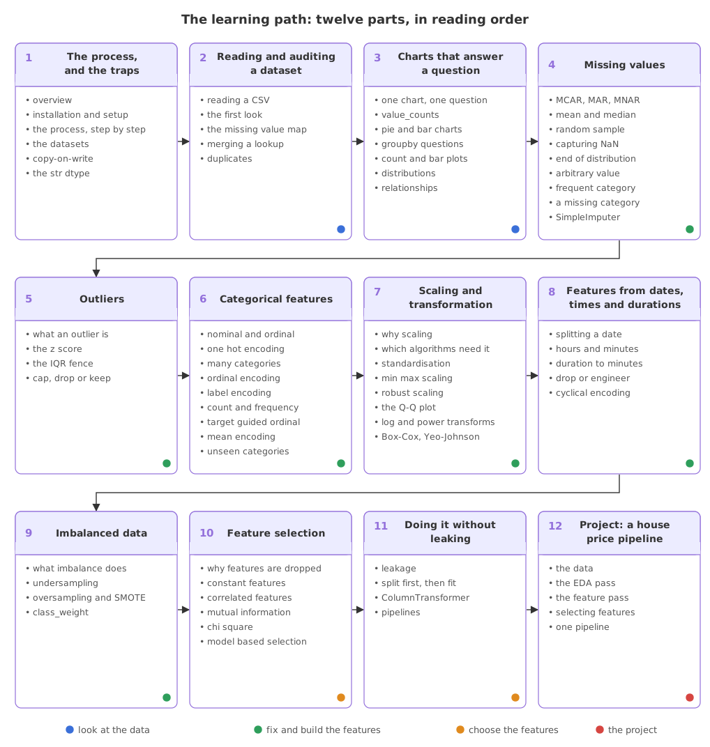
The parts run in the order the work runs in. The first two parts get a dataset into memory and audited, the third charts it, the next five fix and build the columns, the ninth and tenth decide which rows and which columns to keep, the eleventh puts the whole thing behind a train and test split, and the last one builds a house price pipeline out of the pieces.
| Part | Lessons |
|---|---|
| 1. The process, and the traps | EDA and Feature Engineering · Installation and setup · The process, step by step · The datasets this course uses · Copy-on-write and chained assignment · Text columns and the str dtype |
| 2. Reading and auditing a dataset | Reading a CSV that is not UTF-8 · The first look at a dataset · The missing value map · Merging a lookup table · Duplicates |
| 3. Charts that answer a question | One chart, one question, one observation · Counting categories with value_counts · Pie and bar charts with a top-N trim · Answering a question with groupby · Count plots and bar plots in seaborn · Distributions with histograms, KDE and box plots · Relationships between features |
| 4. Missing values | Why values go missing · Mean and median imputation · Random sample imputation · Capturing NaN with an indicator column · End of distribution imputation · Arbitrary value imputation · Frequent category imputation · Missing as its own category · SimpleImputer in scikit-learn |
| 5. Outliers | What an outlier is · Finding outliers with the z score · The IQR fence · Treating outliers by capping or dropping |
| 6. Categorical features | Nominal and ordinal features · One hot encoding · One hot encoding with many categories · Ordinal encoding · Label encoding · Count and frequency encoding · Target guided ordinal encoding · Mean encoding · Handling an unknown category |
| 7. Scaling and transformation | Why features are scaled · Which algorithms need scaling · Standardisation · Min max scaling · Robust scaling · Reading a Q-Q plot · Log, reciprocal and square root transformations · Box-Cox and Yeo-Johnson |
| 8. Features from dates, times and durations | Splitting a date into columns · Turning a time into hours and minutes · Turning a duration string into minutes · When to drop a feature instead of engineering it · Cyclical encoding for hours and weekdays |
| 9. Imbalanced data | What imbalance does to a model · Undersampling · Oversampling and SMOTE · class_weight, and when not to resample |
| 10. Feature selection | Why features are dropped · Dropping constant features · Dropping correlated features · Mutual information · Chi square for categorical features · Model based selection with Lasso |
| 11. Doing it without leaking | Data leakage · Split first, then fit · ColumnTransformer · Pipelines and pandas output |
| 12. Project: a house price pipeline | Project: the house price data · Project: the EDA pass · Project: building the features · Project: the feature selection · Project: the whole thing as one pipeline |
Who this course is for
- Anyone whose model is fine and whose data is the problem. The accuracy is poor, the training will not converge, or a transform raises on the test set and not on the training set.
- Beginners who can call pandas but cannot yet read a dataset. You can plot a chart, and the next question is what the chart tells you to do.
- Interview preparation. The difference between standardisation and normalisation, why mean encoding overfits, what MCAR means and when to use SMOTE are standard questions, and each has a lesson here with a run behind it.
- Anyone following a tutorial recorded before 2023. The code in those notebooks still looks right and no longer does the same thing.
What to know first
- Python basics: variables, lists, dictionaries, functions, loops and importing a library.
- Enough pandas to read a CSV and select a column. Everything beyond
read_csvanddf['col']is explained where it is used. - School statistics: a mean, a median and a standard deviation. Quartiles and the normal distribution are introduced where the outlier and scaling lessons need them.
- A computer with Python 3.12 or newer, or a browser and a Google account for Colab. Installation and setup covers both routes.
- No API keys, no GPU and no downloads. Every dataset is read over the network from a raw GitHub address inside the example itself.
Where the data comes from
Four tables carry the whole course: Titanic (891 rows), the Ames house prices (1460 rows and 81 columns), a mobile price table (2000 rows) and a Mercedes-Benz test-bench table (4209 rows). A Zomato restaurant table carries the reading and charting lessons, and a pair of flight fare spreadsheets carries the lessons on dates and durations. All of them live in the materials repositories listed below and are read by URL, so there is no download step and no copy of the data to keep in sync. The datasets this course uses loads every one of them and prints its shape.
Following the videos and the notebooks
The lessons follow Complete Exploratory Data Analysis And Feature Engineering In 3 Hours, which works through three case studies, and Step By Step Process In EDA And Feature Engineering In Data Science Projects, which sets out the order the steps run in. The techniques that those two leave out come from the live feature engineering sessions and from the notebooks that go with them.
The notebooks are the course notes: 5-Days-Live-EDA-and-Feature-Engineering holds the three case studies, Feature-Engineering-Live-sessions holds the imputation, encoding, scaling and outlier notebooks, Advanced-House-Price-Prediction- holds the house price data and its end to end pass, and Complete-Feature-Selection holds the selection notebooks.
Those notebooks were recorded between 2019 and 2022. Every example in this course has been re-run on the current releases, and these are the calls whose behaviour changed:
| In the notebooks (2019 to 2022) | On pandas 3.0 and scikit-learn 1.9 |
|---|---|
df['Age'].fillna(v, inplace=True) | Fills a temporary copy and leaves the frame untouched. It warns and does not raise |
df[col].dtypes == 'O' | Always False. Text columns use the str dtype, not object |
df1.append(df2) | Removed. pd.concat([df1, df2], ignore_index=True) replaces it |
sns.barplot('x', 'y', data=df) | Raises. Pass x=, y= and data= by keyword |
pd.get_dummies(df, drop_first=True) | Returns bool columns. Pass dtype=int for 0 and 1 |
load_boston() | Removed from scikit-learn. The correlation lesson uses the house price table instead |
sampler.fit_sample(X, y) | Renamed fit_resample, and every imbalanced-learn constructor is keyword only |
Related
- Next: Installation and setup
- Then: The process, step by step
- Notes: the case study notebooks and the technique notebooks on GitHub
- Reference: the pandas user guide and the scikit-learn preprocessing guide
Every expert started right here.